|
|
- ... problem.1
- Here our educators have to solve the
problem of how to test
our problem solving skills instead of our skill in memorizing.
This is a topic for another paper.
.
.
.
.
.
.
.
.
.
.
.
.
.
.
.
.
.
.
.
.
.
.
.
.
.
.
.
.
.
.
- ... reflex1.1
- The siphon
is used to facilitate the snail's breathing. When aplysia breathes, water is
drawn across the gill from the front and exits through the
siphon. The siphon is usually outside of the snail's shell or
mantle. However, when gently touched, the snail will withdraw and
protect its siphon for a short period of time. If this touch is
preceded by an electric shock
to the tail, the snail will withdraw its siphon for a longer period
of time. The snail will continue to have this exagerated response
for up to a day following the shock, and thus, is an example of short
term memory. Multiple shocks given over multiple days cause this
exagerated response to become even more exagerated and retained for
much longer. Even after a week since the electric shocks, the snail
will continue to exhibit the exagerated behavior, and this is an
example of long term memory.
.
.
.
.
.
.
.
.
.
.
.
.
.
.
.
.
.
.
.
.
.
.
.
.
.
.
.
.
.
.
- ... calcium1.2
- We
are assuming calcium, Ca, is the agent responsible for short term memory
because it is probably
critical for neurotransmitter release required to signal adjacent neurons.
More intraceulluar Ca would trigger an increase in the release of
pre-synaptic neurotransmitter which would then activate more post-synaptic
receptors, giving a larger post synaptic response.
.
.
.
.
.
.
.
.
.
.
.
.
.
.
.
.
.
.
.
.
.
.
.
.
.
.
.
.
.
.
- ... potential1.3
- A brief primer in electrophysiology:
Membrane Potential is the result of a difference in the
relative concentrations of positively and negitively charged
particles on opposite sides of a cell's plasma membrane. Cells that
have the ability to maintain an a transmembrane gradient in
charged ions (and thus generate a membrane potentials)
and can rapidly change their
membrane potential following a suprathreshold stimulation are called
excitable cells.
An excitable cell is either in the rest state where the transmembrane
potential is -50 to -80 mV or in the excited state where the
transmembrane potential can become as large as +40 mV for a few
milliseconds. The electrical response to suprathreshold stimulation
is called an action potential (see figure 2.6.3)
and is caused by the rapid influx of
a + charge carrier (either Na or Ca). The restoration of the
charge balance is accomplished by a slower efflux of
a + charge carrier (K) from the intracellular fluid. However, the
charge redistributuion alone is insufficient to keep the cell healthy.
The charge carriers must also be redistributed - which is a regulatory
process that takes place in the background of cellular activity.
Because charge flow during the action potential is down concentration
gradients, it is physically impossible to restore the charge
carriers without active transport up the concentration
gradient by actively exchanging ions between the
extracellular and intracellular fluids. The Na-K transporter is an
example of an active transporter that exchanges extracellular K for
intracellular Na.
.
.
.
.
.
.
.
.
.
.
.
.
.
.
.
.
.
.
.
.
.
.
.
.
.
.
.
.
.
.
- ...
discontinuous1.4
- Our
friend, Valentin Krinsky, was
the first to articulate this
.
.
.
.
.
.
.
.
.
.
.
.
.
.
.
.
.
.
.
.
.
.
.
.
.
.
.
.
.
.
- ... wave1.5
- Spirals form from fragments because the ends
of the fragment propagate more slowly than the interior segments of the wave.
Why? because the ends must excite not only the cells in front of them but
also the cells to the side - and, because the cell has a limited charge
available
to excite adjacent cells, more time is required to transfer this charge
to the larger audience of adjacent cells
.
.
.
.
.
.
.
.
.
.
.
.
.
.
.
.
.
.
.
.
.
.
.
.
.
.
.
.
.
.
- ... -1.6
- This site in the heart is composed of what
are called pacemaker cells
.
.
.
.
.
.
.
.
.
.
.
.
.
.
.
.
.
.
.
.
.
.
.
.
.
.
.
.
.
.
- ... excitability1.7
- Four examples
for such an asymmetry are: inexcitable obstacles that the wave
collides with, cellular coupling, as described by
Maddy Spach, dispersion of refractoriness, or a spatially
inhomogeneous distribution of potassium channels.
.
.
.
.
.
.
.
.
.
.
.
.
.
.
.
.
.
.
.
.
.
.
.
.
.
.
.
.
.
.
- ... switches1.8
- Both excitable cells and DNA
transcription involve switches. Switches are either on or
off. The phase plane of any system with two stable states
requires a third, intermediate state that is unstable and possibly
oscillatory.
.
.
.
.
.
.
.
.
.
.
.
.
.
.
.
.
.
.
.
.
.
.
.
.
.
.
.
.
.
.
- ... gradients2.1
-
In the presence of both an ionic concentration gradient and an electric
field, two currents are possible, one derived from passive diffusion
of charge carriers down the concentration gradient and one derived
from the attraction of a charge carrier by the electric field.
.
.
.
.
.
.
.
.
.
.
.
.
.
.
.
.
.
.
.
.
.
.
.
.
.
.
.
.
.
.
- ... potential2.2
-
The reversal potential is the transmembrane potential
required to create a current based on charge attraction that
exactly balances the diffusive flow of charge carriers down
the concentration gradient.
For example, consider
a higher concentration of Na outside of the cell than inside.
The reversal potential required to stop the diffusive current is
described by
where  is the Rydburg constant, is the Rydburg constant,  is absolute temperature, is absolute temperature,  is
the Faraday constant, is
the Faraday constant,
![$ [\textrm{Na}]_o$](img148.png) is the concentration of Na outside of the cell
and is the concentration of Na outside of the cell
and
![$ [\textrm{Na}]_i$](img149.png) is the Na concentration inside. The equation is
is derived by equating the diffusive current with the current
created by an electric field. A full treatment of this equation can
be found in Appendix D.1. is the Na concentration inside. The equation is
is derived by equating the diffusive current with the current
created by an electric field. A full treatment of this equation can
be found in Appendix D.1.
.
.
.
.
.
.
.
.
.
.
.
.
.
.
.
.
.
.
.
.
.
.
.
.
.
.
.
.
.
.
- ... factor.2.3
-
The specific mechanics of this solving an ordinary differential equation using
an integration factor is fully described in Section 2.10.3.
.
.
.
.
.
.
.
.
.
.
.
.
.
.
.
.
.
.
.
.
.
.
.
.
.
.
.
.
.
.
- ... it.2.4
- See
Section 2.10.1 for a complete overview of the general method of phase plane
analysis.
.
.
.
.
.
.
.
.
.
.
.
.
.
.
.
.
.
.
.
.
.
.
.
.
.
.
.
.
.
.
- ...
unstable2.5
- See Section 2.10.1 for a full explanation of the
terms stable and unstable.
.
.
.
.
.
.
.
.
.
.
.
.
.
.
.
.
.
.
.
.
.
.
.
.
.
.
.
.
.
.
- ... value3.1
- That is, a greater
value, or lesser value, or both,
depending on the model and the type of hypothesis you are testing.
The details of this will be explained in the next few paragraphs.
.
.
.
.
.
.
.
.
.
.
.
.
.
.
.
.
.
.
.
.
.
.
.
.
.
.
.
.
.
.
- ... situations.3.2
- A lot of the material in
this section was plagiarized from the web page: http://www.stat.yale.edu/Courses/1997-98/101/chigf.htm, author unknown.
.
.
.
.
.
.
.
.
.
.
.
.
.
.
.
.
.
.
.
.
.
.
.
.
.
.
.
.
.
.
- ... 1.3.3
- Most
computer languages have standard routines that do this. For example,
rand() in Perl and in C there is rand() and random(), which both return random numbers between 0 and RAND_MAX
.
.
.
.
.
.
.
.
.
.
.
.
.
.
.
.
.
.
.
.
.
.
.
.
.
.
.
.
.
.
- ...
independent3.4
- Independent simply means that knowing the value
of one specific data point does not tell you anything about the value
of any of the other data points. For example, if our data consisted
of the results of tossing a coin, knowing that
 landed heads
would not tell us a thing about whether landed heads
would not tell us a thing about whether  landed heads or tails. landed heads or tails.
.
.
.
.
.
.
.
.
.
.
.
.
.
.
.
.
.
.
.
.
.
.
.
.
.
.
.
.
.
.
- ...X.3.5
- For example, if your
data set was two heads when a coin is tossed twice, then the
probability of the data is
 , since the probability
of getting heads on any one toss is 1/2. , since the probability
of getting heads on any one toss is 1/2.
.
.
.
.
.
.
.
.
.
.
.
.
.
.
.
.
.
.
.
.
.
.
.
.
.
.
.
.
.
.
- ... involved.3.6
- There is a third alternative, called
``variational method'' which is interesting, but I don't quite
fully understand well enough to write about at this time
.
.
.
.
.
.
.
.
.
.
.
.
.
.
.
.
.
.
.
.
.
.
.
.
.
.
.
.
.
.
- ...3.63.7
- For now we will discuss how the
method works for functions of
three variables, but it works fine on functions with two variables (as
you'll see in Example 3.11.1.1) and trivially extends to functions with more.
.
.
.
.
.
.
.
.
.
.
.
.
.
.
.
.
.
.
.
.
.
.
.
.
.
.
.
.
.
.
- ... results.3.8
- Complete derivations of these
results can be found in Appendix D.3 and D.4.
.
.
.
.
.
.
.
.
.
.
.
.
.
.
.
.
.
.
.
.
.
.
.
.
.
.
.
.
.
.
- ...
line3.9
- It is important to note, that just because the data does
not all fall on a single line, doesn't mean that the model is not
linear. There could have been errors in measurement, both human and
mechanical, that cause the data to deviate from a line.
.
.
.
.
.
.
.
.
.
.
.
.
.
.
.
.
.
.
.
.
.
.
.
.
.
.
.
.
.
.
- ... examples.3.10
- However, see
Example 3.13.5.3 for the solution to this current conundrum!
.
.
.
.
.
.
.
.
.
.
.
.
.
.
.
.
.
.
.
.
.
.
.
.
.
.
.
.
.
.
- ... coefficients3.11
- For a function,
 , to be
considered linear with respect to its coefficients means that if the
function were considered to be a function of the coefficients, , to be
considered linear with respect to its coefficients means that if the
function were considered to be a function of the coefficients,
 , then , then
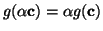 . For
example, the function, . For
example, the function,
 , can be written in terms
of c, , can be written in terms
of c,
 and and
 .
Another example of a function that is linear with respect to its
coefficients is .
Another example of a function that is linear with respect to its
coefficients is
 , because
. An example of a function
that is not linear with respect to its coefficients is , because
. An example of a function
that is not linear with respect to its coefficients is
 , since , since

.
.
.
.
.
.
.
.
.
.
.
.
.
.
.
.
.
.
.
.
.
.
.
.
.
.
.
.
.
.
- ... measurements3.12
- In
Section 3.13.6, Linear Models with Multiple
Dependent Variables we will generalize the test developed here
for multiple dependent variables.
.
.
.
.
.
.
.
.
.
.
.
.
.
.
.
.
.
.
.
.
.
.
.
.
.
.
.
.
.
.
- ... noise.3.13
- I like to use this concept instead
of calling
 ``error'' which it is not. It simply reflects the
limits of our ability to capture the totality of what is going on. With
perfect models, we'd be able to capture the thermal noise generated by
molecular motion and have a perfect fit. So - errors - NO, noise - YES. ``error'' which it is not. It simply reflects the
limits of our ability to capture the totality of what is going on. With
perfect models, we'd be able to capture the thermal noise generated by
molecular motion and have a perfect fit. So - errors - NO, noise - YES.
.
.
.
.
.
.
.
.
.
.
.
.
.
.
.
.
.
.
.
.
.
.
.
.
.
.
.
.
.
.
- ... thus3.14
- We can easily verify that this solution for
 is a minimum by taking the second
derivative of Equation 3.13.4 with respect to is a minimum by taking the second
derivative of Equation 3.13.4 with respect to
 and observing that when and observing that when  is not
completely filled with zeros, the resulting quantity, is not
completely filled with zeros, the resulting quantity,
 , will be positive. , will be positive.
.
.
.
.
.
.
.
.
.
.
.
.
.
.
.
.
.
.
.
.
.
.
.
.
.
.
.
.
.
.
- ... distributed3.15
- It is possible to use
distributions other than the normal as long as each
 is
an independent
variable with mean 0 (zero) and variance is
an independent
variable with mean 0 (zero) and variance  . These
conditions are called Gauss-Markov Conditions. However, when
you use a
normal distribution, the least squares estimates are the same as the
maximum likelihood estimates and are thus best unbiased
estimators, which is a good thing. . These
conditions are called Gauss-Markov Conditions. However, when
you use a
normal distribution, the least squares estimates are the same as the
maximum likelihood estimates and are thus best unbiased
estimators, which is a good thing.
.
.
.
.
.
.
.
.
.
.
.
.
.
.
.
.
.
.
.
.
.
.
.
.
.
.
.
.
.
.
- ... equal3.16
- This would amount to an ANOVA test. See
Example 3.13.5.4 for a full treatment of this.
.
.
.
.
.
.
.
.
.
.
.
.
.
.
.
.
.
.
.
.
.
.
.
.
.
.
.
.
.
.
- ... methods.3.17
- That our solution provides the
maximum probability is easily verified in the manner demonstrated in Example 3.9.2.1
.
.
.
.
.
.
.
.
.
.
.
.
.
.
.
.
.
.
.
.
.
.
.
.
.
.
.
.
.
.
- ... zero3.18
- To see this, all that is needed is to
multiply them out and some minor cancellation. See D.5
for a full derivation of this fact.
.
.
.
.
.
.
.
.
.
.
.
.
.
.
.
.
.
.
.
.
.
.
.
.
.
.
.
.
.
.
- ... to3.19
- See D.6 for a full derivation of
this reduction.
.
.
.
.
.
.
.
.
.
.
.
.
.
.
.
.
.
.
.
.
.
.
.
.
.
.
.
.
.
.
- ...
 3.20 3.20
- Don't worry too much about this, we'll derive the
value for this constant before too long
.
.
.
.
.
.
.
.
.
.
.
.
.
.
.
.
.
.
.
.
.
.
.
.
.
.
.
.
.
.
- ...-distribution 3.21
- An -distribution is defined as the ratio
of two independent chi-square variables, each divided by its degrees
of freedom. That is,
where
 , ,
 and and  and and  are independent.
.
.
.
.
.
.
.
.
.
.
.
.
.
.
.
.
.
.
.
.
.
.
.
.
.
.
.
.
.
.
- ... true.3.22
- Just as a
gentle reminder, the value,
 and the ratio in
Equation 3.13.21 represent points on an and the ratio in
Equation 3.13.21 represent points on an  -axis. The value,
, represents a cut-off point, and anything larger,
and thus further away from the mean, is determined to not come from the same distribution. -axis. The value,
, represents a cut-off point, and anything larger,
and thus further away from the mean, is determined to not come from the same distribution.
.
.
.
.
.
.
.
.
.
.
.
.
.
.
.
.
.
.
.
.
.
.
.
.
.
.
.
.
.
.
- ... model3.23
- This use of the word modern is perhaps
wishful thanking as it is the author's opinion that this model should be
considered thus. In practice, most people, for historical reasons, use
alternative models for ANOVA. See Appendix E, for a full
discussion on this topic.
.
.
.
.
.
.
.
.
.
.
.
.
.
.
.
.
.
.
.
.
.
.
.
.
.
.
.
.
.
.
- ... singular3.24
- This can be
seen by first adding together the first five columns in X,
which will give you a vector of 1s. Adding the last three columns
of X together also gives you a vector of 1s. Thus, adding the
first five columns and subtracting the last three columns will
result in a vector of 0s, satisfying the definition of a singular matrix.
.
.
.
.
.
.
.
.
.
.
.
.
.
.
.
.
.
.
.
.
.
.
.
.
.
.
.
.
.
.
- ... learn.3.25
- A
large number of different interaction plots, as well as their
potential interpretations is given in Appendix F.
.
.
.
.
.
.
.
.
.
.
.
.
.
.
.
.
.
.
.
.
.
.
.
.
.
.
.
.
.
.
- ... are:3.26
- The data given here were stolen from David
Dickey and Jimmy Joi's web page:
http://www.stat.ncsu.edu/
 st512_info/
dickey/crsnotes/notes_5.htm. st512_info/
dickey/crsnotes/notes_5.htm.
.
.
.
.
.
.
.
.
.
.
.
.
.
.
.
.
.
.
.
.
.
.
.
.
.
.
.
.
.
.
- ... is3.27
- See Appendix D.8 for the
derivation
.
.
.
.
.
.
.
.
.
.
.
.
.
.
.
.
.
.
.
.
.
.
.
.
.
.
.
.
.
.
- ... pdf4.1
- xmgrace doesn't do the best job exporting PDF images
so it is sometimes better to export an EPS image an use epstopdf to create the PDF version. You will just have to do it
both ways and decide which looks better.
.
.
.
.
.
.
.
.
.
.
.
.
.
.
.
.
.
.
.
.
.
.
.
.
.
.
.
.
.
.
- ...
computer.4.2
- A lot of the material in this section was
plagiarized from the web page: CVS-RCS-HOWTO.html, written by
Alavoor Vasudevan.
.
.
.
.
.
.
.
.
.
.
.
.
.
.
.
.
.
.
.
.
.
.
.
.
.
.
.
.
.
.
- ... rankD.1
- The rank of a matrix is
the number of linearly independent rows or columns. For any matrix,
the number of linearly independent rows is
equal to the number of linearly independent columns.
.
.
.
.
.
.
.
.
.
.
.
.
.
.
.
.
.
.
.
.
.
.
.
.
.
.
.
.
.
.
| |
![$\displaystyle V_{\textrm{Na}} = \frac{RT}{F} \ln\frac{[\textrm{Na}]_o}{[\textrm{Na}]_i},$](img146.png)