|
to to be the constraint that we use when we try to estimate no_titleno_title
Example 3.13.5.4 (no_title)
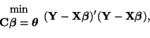
If our model had four parameters and we wanted to test to see if they
were all equal3.16, we would use the following constraint.
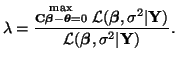
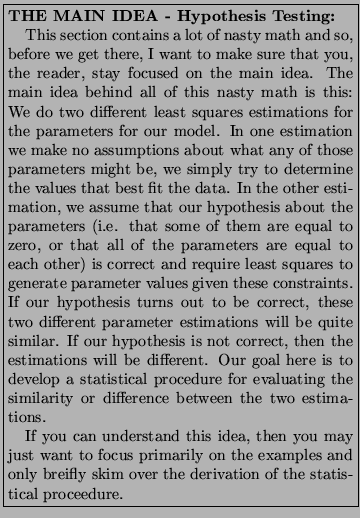
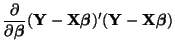
If, given the data, there is a high probability that this system of equations is correct, then all of the parameters must all be equal. In general our hypotheses will take the form We can test our hypotheses by creating a LRT. That is, by comparing the unconstrained optimization of the least squares residual with a constrained optimization of the least squares residual. In Section 3.13.3 we solved for the unconstrained optimization and the result was Equation 3.13.6. To solve for the constrained optimization, that is
we will use the method of Lagrange Multipliers (see Section 3.11 for details on this method). Thus, we want to find solutions to the equations: and or Taking the gradient of Equation 3.13.10, we have
Thus, in terms of We can solve for We can substitute this solution into Equation 3.13.12 giving us the optimal solution for
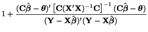
The LRT
for the hypothesis
The constrained and unconstrained estimates for
Now we need to solve for the unconstrained and constrained estimates
of
thus,
Solving for the constrained estimate,
However, in order for it to be usable in a convenient way, we must simplify it and this is quite involved.
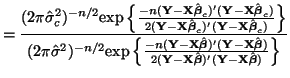
We'll start our simplification of
![\begin{multline*}
({\bf Y} - {\bf X}\hat{\boldsymbol{\beta}}_c)
= {\bf Y} - {\bf...
...ght]^{-1}(\boldsymbol{\theta} - {\bf C}\hat{\boldsymbol{\beta}})
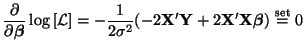
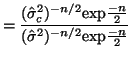
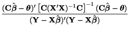
\end{multline*}](img871.png) Thus, While this is formidable, the second and third terms equal zero3.18 and the last term reduces to3.19 If we multiply Equation 3.13.17 by -1 twice, (that is, by 1), we get the equivalent and more common form, Now that we have MLEs for all of the parameters in the model, we can put together a likelihood ratio test. If Equation 3.13.18 is smaller than some constant If we invert our test, then we can reject our hypothesis when it is greater than
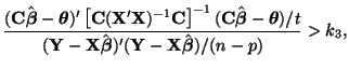
In order to determine what
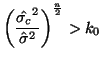
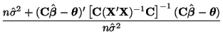
and use algebra to modify both sides until we can recognize the form of the left side. If the form on the left side is a standard distribution, (and in this case, since we have a ratio of variances we'll end up with an
All we have done so far is raise each side of the inequality to the
and where
Since we are able to show that the left hand side of
Equation 3.13.21 has an no_titleno_title
Example 3.13.5.6 (no_title)
Given the Leghorn data in Table 3.13.1 we can try to fit the
model,
![\begin{displaymath}
{\bf Y} =
\left[
\begin{array}{c}
87.1\\
93.1\\
89.8\\
91...
...\
1 & 5.1\\
1 & 5.2\\
1 & 4.9\\
1 & 5.1
\end{array}\right]
\end{displaymath}](img921.png)
To test whether or not body weight is an indicator of food
consumption, that is, whether or not
and the output from our program is: octave:2> general_linear (x, y, [0, 1]); beta = 55.2633 7.6901 f_test = 16.232 p_value = 0.0037939 t_test = 4.0289Thus, since the p-value is much smaller than 0.05, we can conclude that ANOVAno_title
Example 3.13.5.8 (ANOVA)
Given the data in Table 3.13.2,a modern ANOVA model3.23 ![\begin{displaymath}
{\bf Y} =
\left[
\begin{array}{c}
55\\
47\\
46\\
53\\
47...
... & 1 & 0\\
0 & 0 & 0 & 1\\
0 & 0 & 0 & 1
\end{array}\right].
\end{displaymath}](img929.png)
![\begin{displaymath}
{\bf C} =
\left[
\begin{array}{cccc}
1 & 0 & 0 & -1\\
0 & 1 & 0 & -1\\
0 & 0 & 1 & -1
\end{array}\right].
\end{displaymath}](img930.png)
Using our Octave program, we get:
> [x, y] = load_data("mice.dat");
> c = [1, 0, 0, -1;
> 0, 1, 0, -1; 0, 0, 1, -1]
c =

   1   0   0  -1
   0   1   0  -1
   0   0   1  -1

> general_linear (x, y, c);
beta =

  50.250
  45.500
  47.600
  38.500

f_test = 4.3057
p_value = 0.030746
Thus, since our p-value is less than 0.05, we can reject our
hypothesis that there is no difference in the treatment means.
Randomized Block Designno_title
Example 3.13.5.10 (Randomized Block Design)
Sometimes there are extra sources of variation in your data that you can clearly define. For example, in a laboratory, 5 different people may have run the same experiment and recorded their results. We could treat all of the experiments equally, ignoring the fact that we know that 5 different people were involved and just use standard ANOVA for hypothesis testing, or we could try to take into account the fact that some people may be more precise than others when making measurements and that some of the variation in the data may be due to this. The goal of this example is to demonstrate how this second option can work and how we can effectively make use of the extra information at hand. Before we begin, however, we will note that this method only makes sense in specific situations and that, with a little more data, we can use much more powerfull methods for analysis. In this example we are assuming that it would be unreasonable to have each person run the experiment more than once. If this were not the case, we would apply the methods explained in Example 3.13.5.6.
Consider the data set in Table 3.13.3, where we have a
single experiment to compare three different methods for drying leaves
after they have been rinsed performed by five different people.
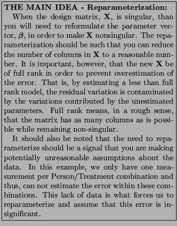
The term Block refers to how randomization was used to set up the experiemental design. Here we are considering each person to represent a block and that within each block, the order in which the different drying methods is applied is randomized. That is to say, Person (Block) #1 may have used the blotting method first, then the control method and then the air current method. Person (Block) #2 may have started with the control method, then used the air current method and then the blotting method. This randomization within blocks is important to make sure that bias is not introduced to the data by where a treatment is applied. It could be that if one treatment was always done last, then it could have a bias due to the student wanting to get done quickly and go home for the evening. For the data in Table 3.13.3, the model is: where
and while Y is fine, X is a singular3.24matrix and we will not be able to invert X'X. A common solution to this problem is to use tricks that are often applied to traditional ANOVA models (ANOVA models that contain a general location parameter or overall mean and the remaining parameters are deviations from that mean) to reparameterize
In order to reparameterize
and thus, and Since we can derive both
and design matrix then becomes
To test the hypothesis that there is
no difference in the treatments is we want to know if the treatment
deviations are all zero. We can create a contrast matrix to directly
test to see if
Using Octave we get:
> general_linear (x, y, c);
beta =

   949.867
   -41.867
    99.467
   -19.867
   -33.867
   -38.067
    18.333

f_test = 0.82474
p_value = 0.47244
and since the p-value is greater than 0.05, we will conclude that there is no difference in the three
treatments. It is worth noting that if we had ignored the blocks and
just used regular ANOVA, than the f-statistic would have been 0.71 and
the p-value would have been 0.5128, demonstrating that by not
ignoring the blocks, we have increased the precision of our test, even
though we would have come to the same conclusion.
If we wanted to test the hypothesis that there was no difference in the different blocks (in this case this would mean that each person applied the treatment in more or less the same way), than we would have to test to see if the block deviations were all zero. Using the same logic used to create the contrast matrix for the treatment hypothesis we have:
Using Octave to calculate an F-statistic and a p-value, we get:
 general_linear (x, y, c);
beta =

   949.867
   -41.867
    99.467
   -19.867
   -33.867
   -38.067
    18.333

f_test = 1.5022
p_value = 0.28882
and once again, we would fail to reject our hypothesis and conclude
that there is no significant difference between the blocks.
At this point it is worth noting that if we had more than one
measurement per person/drying method combination, then we would not
have had to do the reparameterization. With only one measurement per
combination, we are forced to assume that there is no interaction
between the person and the drying method. With more measurements, we
do not have to make this assumption and we would have treated
the data as we would a 5x3 factorial experiment. How this is done is
shown in Examples 3.13.5.6, 3.13.5.7 and 3.13.5.8.
2x2 Factorialno_title
Example 3.13.5.12 (2x2 Factorial)
Sometimes you are interested in testing more than one variable at a time. For example, you might want to do this to determine if there are any interactions between two drugs at different dosages. Such an interaction might prevent the two drugs from being as effective together as they would be taken alone. A doctor might find this information helpful when deciding how to make prescriptions. In this case, you would need to use some type of factorial method to test your hypothesis. In this case, the the different drugs would be called Factors and the different dosages of each drug would be called Levels. If we are interested in only two different dosages per drug, then we would use what is called a 2x2 factorial method (2x2 indicating that there is a total of 4 different drug/dosage combinations). In general, factorial method can be used to determine if there is any interactions between the two factors and if there are none, it can then determine the significance of the effects of the different levels of the factors. In a completely randomized experiement with multiple factors, there is no attempt to impose any type of blocking structure. That is to say, the randomization occurs at the top most level of organization (i.e. we randomly select a level from one factor and apply it with a randomly selected level from another factor). In a blocking design, we first designate the blocks and only randomize within the blocks. The general model used for a 2x2 factorial method where Given the data in Table 3.13.4, we can apply the 2x2 factorial method to determine if there is any interaction between a mouse's age and how much prenatal ethanol its mother consumed when determining how quickly it can learn something new. We might speculate that older mice are going to be slow learners regardless of their prenatal environment, where as young mice might be heavily influenced this factor. We can further validate this hunch by creating what is called an interaction plot, Figure 3.13.3, by plotting the average responses for the adolescent and mature mice given the two different conditions (data from Table 3.13.5). In this case we see the two lines are not parallel and this indicates that the age of the mouse potentially changes the size of the effect that the prenatal environment has on its ability to learn.3.25 Since the model we will be using is a linear model, we can apply our general method for hypothesis testing. Thus, the matrices for Y and X are:
To test if there is interaction effects between the factors, and
Figure 3.13.3 indicates that this is probably the case,
we want to test if the slopes in the plot are equal. That is,
and our Octave program gives us the results: > general_linear (x, y, c); beta = 3.6000 15.6000 6.0000 6.4000 f_test = 35.598 p_value = 1.9738e-05 t_test = 5.9664The tiny p-value confirms the intuition gained from Figure 3.13.3. NxM Factorialno_title
Example 3.13.5.14 (NxM Factorial)
If there are more than two levels per factor, then the only thing that
changes is the number of columns in the design matrix, to account for
the larger number of possible combinations between factors, and the
number of rows in the contrast matrix.
For example, if you were to do a 3x2 factorial, X would have 6 columns and in order to test for interactions, C would require 2 rows. The need for the extra row in C is illustrated in Figure 3.13.4, where the two groups of line segments would need to be tested to see if their slopes are equal.
2x2x2 Factorialno_title
Example 3.13.5.16 (2x2x2 Factorial)
By adding an additional factor, you add an extra dimension to types of
interactions that can take place. Instead of a two dimensional table
to describe the combinations of different levels of different factors,
you now need a three dimensional cube. Additional factors require
additional dimensions. Fortunately for us, however, all of these
extra dimensions can be represented by multiple two dimensional
tables.
Consider the data in Table 3.13.6. If we let Body Fat to be factor A, Gender to be factor B and Smoking History to be factor C, we can represent this data with the model: where
Now that we have the model, the question becomes, how do we test hypotheses about it. Can we use it to determine if Body Fat has an effect of its own on how quickly people get fatigued or is it confounded with the other factors? What about smoking? Do differences in how quickly someone is fatigued depend on all three factors working simultaneously? With carefully formulated contrast matrices we can answer all of these questions. Before we start, however, it is important to understand that you need to begin by looking for the highest order interactions (in this case, the potential three way interaction between the three factors) before testing hypotheses about lower order interactions, which, in turn, need to be investigated before you look at whether or not any particular factor has a main effect (operates on its own). This is because if there are higher order interactions involving the specific factor you are interested in testing for main effects, than the data set is not usable for the kind of hypothesis you have in mind. Despite this, we begin by formulating the contrast matrices to test for main effects. The reason we do this, however, is that once we have the matrices needed to test for main effects, we can use them to derive all of the other contrast matrices required test for any possible higher order interactions. Thus, even though we start by creating the contrasts to test for main effects, we do not use them individually until the very end of the analysis if we use them at all. Consider the data from Table 3.13.7 as it is plotted in Figure 3.13.5. If we assumed that there were no higher order interactions, we could test to determine if Body Fat has a main effect by testing to see if the slopes of the lines between Low and High were zero. We can do this by the usual way by calculating the slopes and then determining if they are significantly different from zero or not. Thus, the contrast matrix for the hypothesis that there is no main effect (the slopes are zero) is: Similarly, to test for whether or not Gender has a main effect, we would want to test for whether or not the slopes in Figure 3.13.6 were zero or not. The hypothesis that there is no main effect is encoded into the contrast matrix: Figure 3.13.7 implies that in order to test for a main effect from Smoking, we must define the contrast matrix as follows: Now, all that we need to do to test hypothesis about any higher order interactions is multiply, column by column, the contrast matrices associated with each factor in the interaction. For example, to test for an interaction between Gender and Smoking, we create the new contrast matrix
This contrast matrix is equivalent to testing whether the slopes of the lines within each graph in Figure 3.13.6 are equal. To test a hypothesis about a three way interaction between Body Fat, Gender and Smoking, we simply multiply the columns of all three main effect matrices together. This contrast matrix is
Intuitively, one can also imagine that this contrast matrix tests to determine if the slopes between the graphs in Figure 3.13.6 are equal (see Figure 3.13.8).
As before, to test our hypotheses we create Y and X
Using our contrast matrix for testing for three way interactions between Body Fat, Gender and Smoking, we can use our Octave program and the output is: > general_linear(x, y, c); beta = 25.967 19.867 19.833 12.133 14.067 16.033 12.067 10.200 f_test = 0.20036 p_value = 0.66043 t_test = 0.44761Since the p-value is much larger than 0.05, we will fail to reject the hypothesis that there is no three way interaction between Body Fat, Gender and Smoking. That is to say, there is no three way interaction between the three factors in the study. Thus, we are free to test hypotheses about any possible two way interactions that might be present. Moving on, we now test for interactions between Gender and Smoking. As described above, we define the contrast matrix: and octave gives us: > general_linear(x, y, c); beta = 25.967 19.867 19.833 12.133 14.067 16.033 12.067 10.200 f_test = 1.1859 p_value = 0.29230 t_test = 1.0890leaving us to conclude that, since the p-value is greater than 0.05, there are no interactions between Gender and Smoking. To test if there are interactions between Body Fat and Smoking, and octave gives us: > general_linear(x, y, c); beta = 25.967 19.867 19.833 12.133 14.067 16.033 12.067 10.200 f_test = 7.7612 p_value = 0.013221 t_test = 2.7859so that we would reject the hypothesis that there is no interaction between Body Fat and Smoking. To test for interactions between Gender and Body Fat, and octave gives us: > general_linear(x, y, c); beta = 25.967 19.867 19.833 12.133 14.067 16.033 12.067 10.200 f_test = 1.4622 p_value = 0.24414 t_test = 1.2092and we would fail to reject the hypothesis that there is no interaction between Gender and Body Fat. Finally, since we have determined that Gender is the only factor that is not in a two interaction, we can determine if has a main effect. To test if the hypothesis is that there is no main effect, the contrast matrix is, as defined above, and octave gives us: > general_linear(x, y, c); beta = 25.967 19.867 19.833 12.133 14.067 16.033 12.067 10.200 f_test = 18.915 p_value = 0.00049705 t_test = 4.3492The small p-value tells us to reject our hypothesis and conclude that there is a main effect for Gender. Blocked 2x3 Factorialno_title
Example 3.13.5.18 (Blocked 2x3 Factorial)
It is possible to combine blocking with the factorial method for
analyzing data. Using blocking implies that you are assuming that
some of the potential interactions do not exist while leaving room for
the possibility with other interactions.
Consider the data in Table 3.13.8. Here we have two
factors, Major and Grade, that have been separated into different
blocks defined by Teacher (the measured value is Score). Notice that just like in Example
3.13.5.5, we only have one measurement for each cell in each block.
This prevents us from using the full models from Examples
3.13.5.6 and 3.13.5.8 that allowed us to test for
all possible interactions. Instead, we are forced to assume that
there is no three way interaction between Teacher, Major and Grade.
However, since we have multiple measurements for each Major/Grade
combination, we can test for two way interactions between these two factors.
Given the restrictions of the data, the model is thus, where As with our previous experience with blocking in Example 3.13.5.5, this equation will lead to a singular design matrix and thus we must reparameterize in much the same way we did before. The only significant difference is how we rewrite the interaction terms. Here, we will use the methods we learned in Example 3.13.5.8, where we built the interaction contrasts from the main effect contrasts. Instead of multiplying each column in contrast matrices, we will multiply the rows that determine which specific combination of Major and Grade a particular score is associated with to create the columns that specify the interaction. Thus, the design matrix is:
where Column 1 is the overall mean, As with the factorial method, we need to evaluate the presence of interaction before we determine the effects of the individual factors. To do this, we make the null hypothesis that there is no interaction. This is equivalent to assuming the parameters associated with Columns 7 and 8 are both equal to zero. The contrast matrix is thus,
Using our Octave program, we test our hypothesis:
> general_linear (x, y, c);
beta =

   84.16667
    1.00000
   -0.16667
   -4.27778
   -5.83333
   -0.33333
    2.61111
    0.44444

f_test = 5.3515
p_value = 0.026292
and, due to the small p-value, reject it.
Since we have concluded that there is indeed interactions between Major
and Grade, we can end our inquiry here.
Split-plot Designno_title
Example 3.13.5.20 (Split-plot Design)
Split-plot designs are simply designs that incorporate multiple levels
of blocking, and thus, only attempt to model a subset of the potential
sources of variation. The more ``split'' you see in the name, like
split-split-plot, of the design, the more levels of blocking there are
in it. In this case, where we are just demonstrating split-plot, we
let one factor determining the blocking at the top level, these blocks
are then divided into two sub-blocks, or plots, with the levels of a
second factor applied to each sub-block. These sub-blocks are then
divided into sub-sub-blocks and the levels of a third factor are
randomly distributed among these units. This is illustrated in Figure
3.13.9.
Consider the data in Table 3.13.9.
The table alone is enough to convince us that any hope we might have to model potential three way interactions is a lost cause. The fact that there is only one measurement per cell rules this out by not giving us enough degrees of freedom to model both a three way interaction and estimate the error. We are forced to simply assume that this type of interaction can not exist. On the other hand, we can model a two way interaction between Field and Variety because we have multiple measurements per level of Variety in each Field. We can also model a two way interaction between Variety and Spacing because, across the different Fields, we can come up with several measurements for each Variety/Spacing combination. Thus, the model is: The more common form of this model is: Since we do not have enough degrees of freedom to estimate all of the parameters in a full model (i.e. we are leaving out the three way interaction term) then we will have to reparameterize the design matrix in the same way we did in Example 3.13.5.9. This gives us a design matrix with sixty rows and twenty columns (thank goodness someone has already gone ahead and written a computer program to generate these for us, [5]). Since this is quite large, I will leave it to your imagination, however, a small bit of it can be found in Appendix B.1. Analysis of the data follows that of any model that contains interaction terms. Start by analyzing those to determine if there is interaction. If not, then test for main effects. If there is, then, you have done your best. The contrast matrix for testing for interaction between Variety and Spacing can be found in Appendix B.2 and the result of our test is:
> general_linear (x, y, c);
beta =

   28.111667
    0.228333
    0.518333
    0.238333
    0.828333
   -1.311667
    2.821667
    0.338333
    0.408333
   -0.311667
    0.018333
   -0.941667
    3.363333
    0.480000
   -1.203333
   -0.728333
    0.853333
    0.220000
    0.436667
   -0.671667

f_test = 1.3051
p_value = 0.28457
and the large p-value lets us conclude that there is no interaction
between Variety and Spacing.
Since spacing is not tied up in another interaction term, like Variety, we can go ahead and test for whether or not it has a main effect. This contrast can be found in Appendix B.3 and octave tells us:
> general_linear (x, y, c);
beta =

   28.111667
    0.228333
    0.518333
    0.238333
    0.828333
   -1.311667
    2.821667
    0.338333
    0.408333
   -0.311667
    0.018333
   -0.941667
    3.363333
    0.480000
   -1.203333
   -0.728333
    0.853333
    0.220000
    0.436667
   -0.671667

f_test = 10.567
p_value =  6.1454e-06
Such a small p-value (far less than 0.05) allows us to conclude that
Spacing does indeed have a main effect on the yield.
We will now test to see if the interaction term Field
> general_linear (x, y, c);
beta =

   28.111667
    0.228333
    0.518333
    0.238333
    0.828333
   -1.311667
    2.821667
    0.338333
    0.408333
   -0.311667
    0.018333
   -0.941667
    3.363333
    0.480000
   -1.203333
   -0.728333
    0.853333
    0.220000
    0.436667
   -0.671667

f_test = 0.61686
p_value = 0.68760
and once again, since the p-value is so large, we will fail to reject
the hypothesis that the interaction term is insignificant.
Now that we have established that both Field and Variety are free of any interaction, we can test to see if they have any main effects. As we might expect Field ends up not having a main effect, but Variety does.
It is worth noting that often times statisticians will modify the
formula used to calculate the F-statistic when they are testing for
main effects for factors whose levels are not randomly applied within
the sub-blocks. Instead of using the Mean Square Error (the
estimation for the overall error in the model) in the denominator,
they will use the mean square of Block ANCOVAno_title
Example 3.13.5.22 (ANCOVA)
Analysis of covariance (ANCOVA) is very similar to ANOVA in that the
models contain indicator variables for the various treatments.
The differences comes from the fact that ANCOVA models also contain
variables that represent continuous data,
like weight or height. These continuous variables are called
covariates because, even though they are not controlled by the
experimenter, they are expected to have an influence on the response
to the treatments. You can imagine how heavy and light people might
have different response to different ``treatments'' of alcohol.
Oftentimes there are possible interactions between the covariates and the treatments. For example, if we were trying to determine if two different brands of fertilizer resulted in the same crop yield or not and we were measuring insect infestation as our covariate. We would expect that the greater the infestation, the less crop yield. Beyond this, it could be that one of the fertilizers contained something that insects enjoyed eating and thus, would be more susceptible more substantial infestations. It would then be difficult to tell if low crop yield for this fertilizer would be result of the fertilizer simply not working or due to the fact that the crop was eaten by the insects. Thus, or analysis of covariance begins much the same way as it did for the blocking designs and the factorial data. We start by testing for interactions between the covariate and treatments. Using our example of two fertilizers and insect infestation, the model that leaves interaction as a possibility is, where Fertilizer A and B are dummy 0/1 indicator variables exactly like the ANOVA model and Infestation A and B are infestation values measured for the different treatments (infestation is scored from 0 to 10, with 0 being no infestation and 10 being the most infestation). Given 8 measurements for each treatment, the response vector and the design matrix are:3.26
We can test for interaction by testing whether the Infestation slopes are the same for the different fertilizers. That is, and our general linear models program give us the results: > general_linear (x, y, c); beta = 17.86079 14.48320 -0.67178 -0.59096 f_test = 0.56192 p_value = 0.46793 t_test = 0.74961Here the p-value is much larger than our 0.05 cut off, so that we will fail to reject our hypothesis that the slopes for the covariate given different treatments are different and thus, we can assume that there is no interaction between Infestation and Fertilizer. Since we can ignore interaction, we can use a simpler model (one that leaves out the possibility for interaction) to test whether or not the fertilizers have the same effect on crop yield. This model simply lumps the two Infestation variables into one. We can do this because we failed to detect any difference between the two variables in the more complex model. Thus, our new model is: and the design matrix becomes:
The contrast matrix for determining if there is a difference between the treatments is and our program gives us the results: > general_linear (x, y, c); beta = 14.48603 11.51397 -0.62940 f_test = 60.644 p_value = 2.9992e-06 t_test = 7.7874Such a small p-value causes us to reject the hypothesis that both Fertilizer treatments are the same.
NOTE: This second test, where we have lumped the covariate into
a single variable for all of the treatments in the model and are
testing for differences between the treatments, is equivalent to
conducting the test under the adjusted treatment means
hypothesis that is sometimes mentioned in other statistics texts.
Categorical Datano_title
Example 3.13.5.24 (Categorical Data)
Ever since 1969, linear models have been used to analyze categorical
data [6].
Next: Linear Models with Multiple Up: Linear Models Previous: Properties of Index Click for printer friendely version of this HowTo Frank Starmer 2004-05-19 | ||||||||||||||||||||||||||||||||||||||||||||||||||||||||||||||||||||||||||||||||||||||||||||||||||||||||||||||||||||||||||||||||||||||||||||||||||||||||||||||||||||||||||||||||||||||||||||||||||||||||||||||||||||||||||||||||||||||||||||||||||||||||||||||||||||||||||||||||||||||||||||||||||||||||||||||||||||||||||||||||||||||||||||||||||||||||||||||||||||||||||||||||||||||||||||||||||||||||||||||||||||||||||||||||||||||||||||||||||||||||||||||||||||||||||||||||||||||||||||||||||||||||||||||||||||||||||||||||||||||||||||||||||||||||||||||||||||||||||||||||||||||||||||||||||||||||||||||||||||||||||||
![$\displaystyle \left[ \begin{array}{ccccc} 0 & \ldots & 1_i & \ldots & 0 \end{ar...
...gin{array}{c} \beta_1 \vdots \beta_i \vdots \beta_p \end{array} \right]$](img830.png)
![$\displaystyle \left[ \begin{array}{cccc} 1 & 0 & 0 & -1 0 & 1 & 0 & -1 0 & ...
...eft[ \begin{array}{c} \beta_1 \beta_2 \beta_3 \beta_4 \end{array} \right]$](img832.png)
![$\displaystyle = \left[ \begin{array}{c} 0 0 0 \end{array} \right]$](img833.png)
![$\displaystyle \left[ \begin{array}{c} \beta_1 - \beta_4 \beta_2 - \beta_4 \beta_3 - \beta_4 \end{array} \right]$](img834.png)
![$\displaystyle = \left[ \begin{array}{c} 0 0 0 \end{array} \right].$](img835.png)
![\begin{multline}
\hat{\boldsymbol{\beta}}_c = \boldsymbol{\hat{\beta}}\\
+ ({\b...
...C}']^{-1}(\boldsymbol{\theta} - {\bf C}\hat{\boldsymbol{\beta}}).
\end{multline}](img859.png)
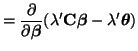
![$\displaystyle \frac{\partial}{\partial \sigma^2}\log\left[ \mathcal{L} \right] ...
...eta}})'({\bf Y} - {\bf X}\hat{\boldsymbol{\beta}})\stackrel{\mathrm{set}}{=} 0,$](img867.png)


![$\displaystyle \left[ \begin{array}{cc} 0 & 1 \end{array} \right] \left[ \begin{array}{c} \beta_0 \beta_1 \end{array} \right]$](img925.png)
![$\displaystyle {\bf Y} = \left[ \begin{array}{c} 950 857 917 887 1,189\\...
... 0 & 0 & 0 & 1 & 0 & 1 & 0 0 & 0 & 0 & 0 & 1 & 0 & 0 & 1 \end{array} \right],$](img941.png)


![$\displaystyle \boldsymbol{\beta} = \left[ \begin{array}{c} \mu \Delta b_1 \...
... b_3 \Delta b_4 \Delta t_1 \Delta t_2 \Delta t_3 \end{array} \right].$](img952.png)
![$\displaystyle {\bf X} = \left[ \begin{array}{rrrrrrr} 1 & 1 & 0 & 0 & 0 & 1 & 0...
...1 & -1 & -1 & -1 & 0 & 1 1 & -1 & -1 & -1 & -1 & -1 & -1 \end{array} \right].$](img953.png)
![$\displaystyle {\bf C} = \left[ \begin{array}{ccccccc} 0 & 0 & 0 & 0 & 0 & 1 & 0 0 & 0 & 0 & 0 & 0 & 0 & 1 \end{array} \right].$](img956.png)
![$\displaystyle {\bf C} = \left[ \begin{array}{ccccccc} 0 & 1 & 0 & 0 & 0 & 0 & 0...
... 0 0 & 0 & 0 & 1 & 0 & 0 & 0 0 & 0 & 0 & 0 & 1 & 0 & 0 \end{array} \right].$](img957.png)
![\includegraphics[width=3in]{2x2_factorial}](img959.png)
![$\displaystyle {\bf Y} = \left[ \begin{array}{c} 5 4 3 4 2 6 7 5\\...
... 0 & 0 & 1 0 & 0 & 0 & 1 0 & 0 & 0 & 1 0 & 0 & 0 & 1 \end{array} \right],$](img962.png)
![\includegraphics[width=3in]{3x2_factorial}](img965.png)
![\includegraphics[width=3in]{maleFS}](img971.png)
![\includegraphics[width=3in]{femaleFS}](img972.png)
![\includegraphics[width=3in]{low_fatBC}](img974.png)
![\includegraphics[width=3in]{high_fatBC}](img975.png)
![\includegraphics[width=3in]{low_fatGS}](img977.png)
![\includegraphics[width=3in]{high_fatGS}](img978.png)
![$\displaystyle = \begin{array}{rrrrrrrrrl} \left[ \right. & -1 & -1 & 1 & 1 & -1...
...left[ \right. & 1 & -1 & -1 & 1 & 1 & -1 & -1 & 1 & \left. \right]. \end{array}$](img981.png)
![$\displaystyle = \begin{array}{rrrrrrrrrl} \left[ \right. & -1 & -1 & -1 & -1 & ...
...left[ \right. & -1 & 1 & 1 & -1 & 1 & -1 & -1 & 1 & \left. \right]. \end{array}$](img982.png)
![\includegraphics[width=3in]{2way}](img983.png)
![\includegraphics[width=3in]{3way}](img984.png)
![$\displaystyle {\bf Y} = \left[ \begin{array}{c} 24.1 29.1 24.6 17.6 18....
...& 0 & 0 & 0 & 0 & 0 & 0 & 1 0 & 0 & 0 & 0 & 0 & 0 & 0 & 1 \end{array} \right]$](img985.png)
![$\displaystyle {\bf X} = \left[ \begin{array}{rrrrrrrr} 1 & 1 & 0 & 1 & 1 & 0 & ...
...& -1 & 0 & 1 & 0 & -1 1 & -1 & -1 & -1 & -1 & -1 & 1 & 1 \end{array} \right],$](img998.png)
![$\displaystyle {\bf C} = \left[ \begin{array}{cccccccc} 0 & 0 & 0 & 0 & 0 & 0 & 1 & 0 0 & 0 & 0 & 0 & 0 & 0 & 0 & 1 \end{array} \right].$](img1000.png)
![\includegraphics[width=2.8in]{split_plot_fig1}](img1001.png)
![\includegraphics[width=2.8in]{split_plot_fig2}](img1002.png)
![\includegraphics[width=2.8in]{split_plot_fig3}](img1003.png)
![$\displaystyle {\bf Y} = \left[ \begin{array}{c} 18 15 12 11 13 17 1...
...& 1 & 0 & 1 0 & 1 & 0 & 0 0 & 1 & 0 & 6 0 & 1 & 0 & 9 \end{array} \right]$](img1022.png)
![$\displaystyle {\bf X} = \left[ \begin{array}{cccc} 1 & 0 & 0 1 & 0 & 5 1 & ...
... 0 & 1 & 0 0 & 1 & 1 0 & 1 & 0 0 & 1 & 6 0 & 1 & 9 \end{array} \right].$](img1027.png)