Next: Model Approximations and Assumptions
Up: How to create a
Previous: Ordinary Differential Equations
Index
Click for printer friendely version of this HowTo
We shall start with the Hodgkin-Huxley equations that describe the
excitable process of a giant squid axon. Although much of what follows
is our speculation, we suspect that our rationale for each equation is quite
similar to theirs.
The equations that we are about to derive are based on
the definitions of the current-voltage relationship for different
circuit components. Combining circuit elements alters the total
current-voltage relationship, and hence, the behavior of the circuit.
Here we use  to be the potential difference across the circuit
element,
to be the potential difference across the circuit
element,  to be the current,
the amount of charge,
to be the current,
the amount of charge,  , that flows per unit
time through the element. , and are functions of both time,
, that flows per unit
time through the element. , and are functions of both time,  and space,
  .
.
- Ohm's Law:
 , where
  is the
conductance (the reciprocal of
is the
conductance (the reciprocal of  , resistance) and represents the proportionality
constant relating current to the difference in potential across
a resistor. This implies that
the current through a resistor is linearly proportional to the
difference in potential across the resistor (the relationship used
to describe current through conducting membrane ion channels).
, resistance) and represents the proportionality
constant relating current to the difference in potential across
a resistor. This implies that
the current through a resistor is linearly proportional to the
difference in potential across the resistor (the relationship used
to describe current through conducting membrane ion channels).
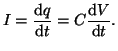
- Definition of Capacitance:
 , where
  is the
capacitance of the circuit element and is the proportionality
constant relating charge with potential.
This implies that the charge stored within a capacitor is
linearly proportional
to the difference in potential across the capacitor.
is the
capacitance of the circuit element and is the proportionality
constant relating charge with potential.
This implies that the charge stored within a capacitor is
linearly proportional
to the difference in potential across the capacitor.
- Current is the amount of charge that flows/unit time so taking
derivatives of the above, we have:
Circuits are constructed by parallel or series combinations of
resistors, capacitors and inductors, however, there are few
biological analogs of inductors and we will ignore them in this
context. The differential equations that
describe the behavior of a circuit are derived by applying
Kirchoff's conservation laws to the circuit:
- Kirchoff's Current Law: All of the current that flows into
a node (an intersection of 2 or more circuit elements) must be equal
to the amount of current that flows out of the node. For example, if
a circuit element has one input and two outputs and one amp flows into
it, then one amp must be distributed between the two outputs.
- Kirchoff's Voltage Law: The sum of the voltage differences
measured around a loop of circuit elements must be zero.
Applying these principles to biological systems yields equations
that can often characterize a surprisingly large amount of behavior.
The fun of modeling is to identify the minimal model required to
capture the behavior of a biological process.
In studies of the relationship between current passing across the
membrane of a squid giant nerve axon,
H-H observed two major currents in response to a step change
in the transmembrane potential, an inward Na current that rapidly
turned on (activated) and off (inactivated), and a slowly activating
outward K current (delayed rectifier) as shown in figure
2.5.1.
They incorporated a third current, a leakage current, in order to
maintain a balance of current under rest conditions.
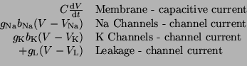
Figure:
Computed ionic currents for squid giant axon.
![\includegraphics[width=3in]{hh_current}](img145.png) |
Each current was characterized by Ohm's law, , but because the
ionic currents flowed according to different gradients2.1, the potential,
, must
be related to the reversal potential2.2,  , where
  is simply a label for the type of current.
The
total current is thus the sum of two components, the field component,
is simply a label for the type of current.
The
total current is thus the sum of two components, the field component,
 and the ion gradient component,
 . Combining the two
we can write Ohms law as
. Combining the two
we can write Ohms law as
The effect of the gradient current
can be seen in Figure 2.5.3 where the Na current goes from being
negative to positive when the potential is a little over +40 mV.
Thus, the reversal potential for Na is +40 mV. For K, the reversal
potential is about -80 mV. The sign and the strength of the
reversal potential is determined by the different gradients of
ions.
H-H considered the membrane as an insulator
surrounded on each side by a conductor (extracellular and intracellular fluid).
Thus, the membrane acts as a capacitor where the amount of charge that can
be stored on the insulating surface is .
Postulating that
the membrane is composed of ion channels that control ion flow between the
extracellular and intracellular fluids, the equivalent electrical
circuit is the parallel combination of a capacitor, the membrane, and 3 conductances,
Na, K and leakage. The current associated with each component of the circuit
can be represented by the terms:
where
 and
and
 are the gating terms and
represent the fraction of
ion channels that are open at a given time. Thus, if all of the Na
channels are open, then
are the gating terms and
represent the fraction of
ion channels that are open at a given time. Thus, if all of the Na
channels are open, then
 and you get full
conductance for Na. However, if only half of the channels are open,
the conductance is scaled by one half.
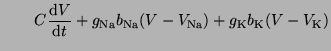
From Kirchoff's current law, the sum of currents flowing into
and out of a node (where circuit element are connected) is zero,
we have
and you get full
conductance for Na. However, if only half of the channels are open,
the conductance is scaled by one half.
From Kirchoff's current law, the sum of currents flowing into
and out of a node (where circuit element are connected) is zero,
we have
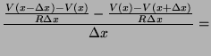
To extend the model to include propagation, unidirectional movement of
ions from cell to cell, we have to add two additional
sources of current in this balance, diffusive current into the
node and diffusive current out of the node. The current into the node
is
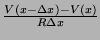 , where is the
internal resistance per unit length (the reciprocal of , conductance). It
is easy to imagine that throughout the length of a cell that there
would be all sorts of obstacles such as intracellular organs or
proteins in the cytosol that would inhibit the free flow of ions
through the cell. Since this hindrance is relatively uniform for the
different types of ions, we only need on term to account for them. The current out of the node
is
, where is the
internal resistance per unit length (the reciprocal of , conductance). It
is easy to imagine that throughout the length of a cell that there
would be all sorts of obstacles such as intracellular organs or
proteins in the cytosol that would inhibit the free flow of ions
through the cell. Since this hindrance is relatively uniform for the
different types of ions, we only need on term to account for them. The current out of the node
is
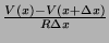 .
Because we cannot manufacture charge, then
the difference per unit length must equal the current through the membrane.
.
Because we cannot manufacture charge, then
the difference per unit length must equal the current through the membrane.
Figure:
Flow of diffusive and ionic current within a nerve or cardiac cell. Ionic
currents flow down a potential gradient along the radial axis of a
nerve or muscle cell, and, as membrane ion channels open, ions can
flow down transmembrane concentration and potential gradients. Typically
Na and Ca ions flow into the cell while K ions flow out of the cell.
![\includegraphics[width=3in]{hh_fig}](img164.png) |
Taking the limit as  goes to zero then we have the standard
nonlinear parabolic partial differential equation with the driving function
composed of the individual ionic currents.
goes to zero then we have the standard
nonlinear parabolic partial differential equation with the driving function
composed of the individual ionic currents.
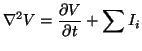 |
(2.5.1) |
where
 ,
,
 and
and
 .
.
At this point, the two gating variables,
and
, were defined by words, but there was no formula to
define their value.
These
gating parameters
separate the H-H model from pure first principles, Ohm's law and
conservation of charge.
This is where
Hodgkin and Huxley strayed from ordinary science to extraordinary
science and this yielded
a Nobel prize.
Hodgkin and Huxley's experiments
revealed that when they switched the potential across the cell membrane
from a polarized value (-60 mV) to a depolarized value, 0 mV, and
they poisoned the K charge carriers so that they saw only
Na current, the Na current decreased
transiently and then returned to zero (or near zero) (the red trace in
Figure 2.5.1).
This feature probably
led them to conjecture that there was some sort of dynamic gating process
that controlled the flow of ions through the channel. For Na current,
they initially suggested two gates, one for activation and one for
inactivation. Similarly for potassium, they initially suggested a
single activation gate (the green
trace in Figure 2.5.1).
To test their model they must have plotted observed and
expected currents. From these plots they would have
observed that the first draft of the model did not fit the initial onset of
the activation process for Na or K.
For Na current, three
activation
gates resulted in a better fit.
The result was that they defined
 ,
where
,
where  is the probability that an activation gate opens after the
nerve is stimulated, thus
is the probability that an activation gate opens after the
nerve is stimulated, thus  is the probability that three open,
and
is the probability that three open,
and  is the probability the inactivation gate slowly closes after
the nerve is
stimulated.
Similarly for the
potassium current, they found that four gates fit the onset of activation
better than a single gate and thus,
is the probability the inactivation gate slowly closes after
the nerve is
stimulated.
Similarly for the
potassium current, they found that four gates fit the onset of activation
better than a single gate and thus,
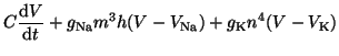
 . Substituting terms, our final equation is:
and the results are shown in Figure 2.5.4
where we show the computed action potential and the three gating variables.
Figure:
Comparison of a single and 3 activation gates for cardiac Na channels.
Experimentally observed peak currents shown as +, single gate as red
and 3 gates as blue
![\includegraphics[width=3in]{iv_gate}](img180.png) |
This curve fitting exercise is a wonderful example of
paying attention to small details. The current voltage relationship
of a Na channel is usually measured by holding the cell at some negative
(-120 mV) potential and then testing the response with a short duration
(5 ms) shift in potential to a test potential. The peaks of each response
is plotted and then you think about what the I/V curve is trying to tell you.
Shown in 2.5.3 are peak
Na currents measured in cultured cardiac cells by Gus Grant (+) as
a function of the test potential and fits to the
I/V curve assuming one (red) and 3 (blue) activation gates. Note that
for the initial activation between -60 mV and -45 mV, the red (single)
curve overestimates the current while the blue curve is right on the money.
Similarly, the single activation gate overestimates the peak of the curve.
Such consistent overestimation is typically not due to noise, but
would suggest that something is missing from the model.
In the H-H days of desk-top calculators, many (probably including me) would
have been happy to get general agreement between observed currents and
model currents as shown by the red line, but not Hodgkin and Huxley.
They must have realized that there was something not quite right and
redid their analysis for a 3 gate process for the Na channel and a
4 gate processes for the K channel.
Figure:
Computed squid action potential and gating variables.
![\includegraphics[width=3in]{hh_gates}](img181.png) |
The first hint that the theory developed by H-H
was correct came about 30 years later when the Na channel
was cloned and sequenced by Noma and colleagues in Japan.
They observed 4 subunits, each with 6 membrane spanning
components
and a perfect arrangement for
a helical gate.
50 years later,
Ray MacKinnon and colleagues managed to crystallize K channels and
found four paddles that acted as voltages sensors for the gating
process.
Next: Model Approximations and Assumptions
Up: How to create a
Previous: Ordinary Differential Equations
Index
Click for printer friendely version of this HowTo
Frank Starmer
2004-05-19