Next: Why It Works
Up: How to ask questions
Previous: Degrees of Freedom
Index
Click for printer friendely version of this HowTo
In the study of genetics one frequently runs into situations that are resolved
using what is called a Chi-Square Goodness of Fit Test. This is a
test that is particularly adept at determining how well a model fits
observed data. It allows us to evaluate how ``close'' the observed
values are to those which would be expected given the model in question. Here is a
brief explanation of how and why the Chi-Square Goodness of Fit Test
is effective in these situations.3.2
In general, the chi-square test statistic has the form:
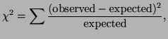 |
(3.7.1) |
and if  is large, than the model is a poor fit to the data.
Before we get into the details of the theory behind this statistic,
let's begin with a short example of how it is used.
is large, than the model is a poor fit to the data.
Before we get into the details of the theory behind this statistic,
let's begin with a short example of how it is used.
A Fair Coin?no_title
Imagine trying to determine if a coin is fair or not. If the coin is
fair, than the probability of getting heads is  and the
probability of getting tails is
and the
probability of getting tails is  , other wise
 and
and
 . It is important to note
that since the coin has only two sides,
. It is important to note
that since the coin has only two sides,
 . While
this equality may seem obvious, it will be useful when we are determining the
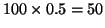
degrees of freedom for our test. If we tossed the coin 100 times, we
would expect to get
heads
. While
this equality may seem obvious, it will be useful when we are determining the
degrees of freedom for our test. If we tossed the coin 100 times, we
would expect to get
heads
 times. We know, however, that even though
the probability of getting heads is
times. We know, however, that even though
the probability of getting heads is  , there is a chance that we
might get a few more or a few less than 50 heads in 100 tosses. The
question is, how much variation in the number of heads will we allow
before we are confident in rejecting the hypothesis that
, there is a chance that we
might get a few more or a few less than 50 heads in 100 tosses. The
question is, how much variation in the number of heads will we allow
before we are confident in rejecting the hypothesis that  ?
This is where the Chi-Square Goodness of Fit comes in handy.
?
This is where the Chi-Square Goodness of Fit comes in handy.
In order to test the hypothesis that the coin is fair, you toss the
coin 100 times and observe that it landed on heads 38 times. From
this data alone, we are able to determine that the coin must have
landed on tails 62 times and we note this in Table 3.7.1.
Table 3.7.1:
Both observed and expected results of 100 coin tosses.
| |
Observed |
Expected |
| Heads |
38 |
50 |
| Tails |
62 |
50 |
|
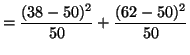
With this data in our hands, we can compute a test statistic
and use it to determine the fairness of the coin.
That is,
We can now see where this values lies in a
distribution. If it is in the tail of the distribution, then
the probability of getting 37 heads using a fair coin would appear to
be a very rare event. If it is in the middle of the distribution,
then it might be quite common to obtain 38 heads in 100 tosses from a
fair coin.
In order to examine our value in the context of a
distribution we must specify
which one by determining its degrees of freedom. We
calculate the total degrees of freedom by looking at the
total number of parameters in our model, 2 ( and
and  ), and
subtracting 1 because is not independent from since
. Thus, we must see how much area is under the curve of a
), and
subtracting 1 because is not independent from since
. Thus, we must see how much area is under the curve of a
 distribution (the subscript 1 indicates the degrees of
freedom) from 5.75 to
distribution (the subscript 1 indicates the degrees of
freedom) from 5.75 to  . We can do this easily using Octave:
octave:1> 1 - chisquare_cdf(5.76, 1)
ans = 0.016395
The probability that a value of 5.76 or larger would come from
the distribution is less 0.016395, which is very small (see
Figure 3.7.1).
Much smaller than the standard 5 percent used as a cutoff to determine
whether we should accept 5.76 as coming from the
distribution. Thus, we will reject the hypothesis that this coin is fair.
Figure:
The area under the graph that represents the p-value, the probability
our hypothesis that the coin is far is correct. Since the p-value/area is so
small (1.6 percent) we will reject our hypothesis.
![\includegraphics[width=3in]{chi_square1}](img540.png) |

Subsections
Next: Why It Works
Up: How to ask questions
Previous: Degrees of Freedom
Index
Click for printer friendely version of this HowTo
Frank Starmer
2004-05-19