The Vulnerable Period: Cardiac and other excitable mediaI am continuing explorations of the vulnerable period, what I assert is a generic property associated with wave motion in an excitable media, how it can be augmented by altering excitability - e.g. with ion channel blockade (guarded receptor model) in cardiac cells: (BZ, cardiac, FHN etc) and how reentrant fronts produce Monomorphic and Polymorphic ECGs
The notion of a vulnerable region in an excitable medium[8.16.2007] For 17 years I've been struggling with how to conceptualize the concept of a vulnerable region. In the early 1990s, I characterized it as a region trailing an excitation wave where stimulation produced a discontinuous wave. This idea persisted until recently when I was challenged as to whether this was a generic property of all excitable media. I suddenly realized that the difference between a non-vulnerable region and a vulnerable region was tied to excitability.
 A little background. A uniformly excitable medium is not
vulnerable. Any disturbance will propagate away from the site of excitation.
When the distrubance exceeds that of the
critical nucleus , the propagation is sustained. When the
disturbed region is less than the critical nucleus, the wave
decrementally propagates and collapses.
A little background. A uniformly excitable medium is not
vulnerable. Any disturbance will propagate away from the site of excitation.
When the distrubance exceeds that of the
critical nucleus , the propagation is sustained. When the
disturbed region is less than the critical nucleus, the wave
decrementally propagates and collapses.
As the excitability is reduced, the critical nucleus increases in amplitude
as shown here. Shown are the critical nuclei for constant inhibitory currents
where the larger the value, the greater the peak of the critical nucleus.
A more excitable region requires a a smaller critical region to initiate a sustained propagating wave that a less excitable medium. Here using the Fitzhugh-Nagumo model with no inhibitory process (trigger wave) one can see the collapse of a pulse to that of the critical nucleus and the resulting propagation. The animation to the right illustrates the concept of the critical nucleus. The amplitude of both the red and blue pulses is larger than the single cell threshold (black line). The red pulse excites a region less than the critical nucleus and collapses. The blue pulse, on the other hand, excites a region larger than the critical nucleus and expands. Now consider a medium with a linear excitability gradient. Disturbing a region in this medium where the excited region is slightly larger than the critical nucleus required in the direction of greater excitability will only decrementally propagate in the direction of lesser excitability. Below is a demonstration of the two cases - uniform excitability and a linear gradient of excitability.
So what is a vulnerable region? Behind every propagating wave is a wake of excitable media whose excitability increases as you move further along the wave back, a result of the gradient of excitability associated with membrane repolarization. For cardiac cells the gradient is produced by the recovery from Na channel inactivation. The gradient can also be produced by use-dependent drugs, a result of unbinding while channels are in the rest state. Consequently, stimulation at a particular point with stimulation parameters such that the critical nucleus is exceeded in the retrograde direction while the excited region is less than the critical nucleus in the antegrade direction will produce a unidirectional propagating wave. This region is referred to as a vulnerable region. [11.27.2002] Since our studies of the vulnerable period in the early 90s, I was puzzled by why use-dependent drugs created a larger vulnerable period than simply reducing the Na conductance. While plotting excitability (in this case, h*j*(1-b) where b is the fraction of blocked channels and h and j are the fast and slow Na channel inactivation, I realized that the gradient of excitability influenced the vulnerable period. The following two papers describe these numerical experiments:
[2.24.2002] The recent observations that some mutations of SCN5A sodium channel lead to loss of function - by slowing the recovery from channel inactivation (which also leads to a hyperpolarizing shift in the inactivation curve) shares a common feature with other proarrhythmic substrates such as ischemia and hyper kalemia. All result in an apparent loss of maximum macroscopic Na conductance. Below I show that the gradient of Na channel availability alters the vulnerable period. A simple reduction in maximal gNa will reduce the gradient and thus prolong the period of vulnerability. This gradient is also influenced by the recovery of Na channel loss of function - either as recovery from inactivation or from recovery from use-dependent channel blockade. Thus, loss of Na channel function - either by a reduction in Na channel density, depolarization of the rest potential, slow the recovery from inactivation - prolongs the period of vulnerability and amplifies the likelihood that a PVC will initiate reentrant activation.
What is the vulnerable period?[3.1.2001] What follows is a bit like brownian motion - old stuff with new ideas - but there is no flow - so excuse me for this. Valentin Krinsky has pushed me to put together some old and new ideas and so there is a new manuscript: How Antiarrhythmic Drugs Increase the Rate of Sudden Cardiac Death. Also, as part of Krinsky's assignment, I made some new numerical studies of the VP, and observed that the duration of the VP depended on the spatial gradient of excitability .]
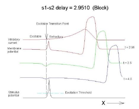
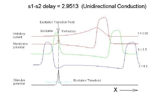
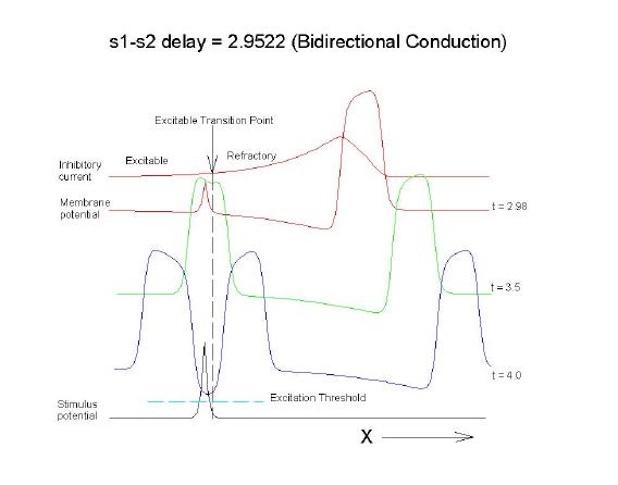
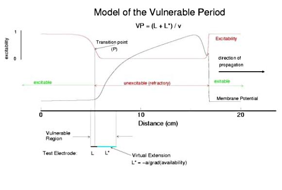
This is an interval of time between regular excitations of the heart, where a stimulus can initiate a self-sustained disturbance to the normal heart rhythm - that can often lead to sudden cardiac death. Originally observed by Mines and later by Ferris and King (see bibliography) the vulnerable period became well known, although the underlying mechanism was not understood. The underlying mechanism has now been identified as the interaction between the "wake" of a front of excitation and a stimulus placed at a critical location and time within this wake. The location and timing depend on the boundary that separates refractory cells from excitable cells - and this is demonstrated below. Click on this link for ideas about the origins of the vulnerable period I illustrate the 3 classes of conditions in a one-dimensional model. using both the Fitzhugh-Naguma model, a simple 2 current model of an excitable cell and the Beeler Reuter model. Many folks dislike this model because it makes a non-biological action potential. I like it because it reduces the complexity of the underlying processes to an absolution minimum. Because the cell membrane separates two pools of charge carriers, there can only be 2 currents, one flowing into the cell and one flowing out of the cell. Consequently, I view "realistic" models as interesting, and able to demonstrate an action potential similar to that seen in experiments. But all the currents embedded in the "realistic" models are simply complex mechanisms for modulating the net current - because in the end, the net flow of charge is either into or out of the cell. I've reproduced the below demonstrations with the Beeler Reuter model, the Beeler-Reuter model using the Ebihara Johnson sodium model, the Lou Rudy model and the Hodgkin-Huxley model. All reveal the essential properties of an excitable cell: a threshold of excitability, a refractory period, a vulnerable period and propagation. The vulnerable period is easily understood by recognizing that there is a "critical" point in the recovery of cellular excitability that separates the "excitable" state from the "refractory" state. I refer to this below as the Excitable Transition Point. When this point falls within the excitation field of an external stimulus, conduction will fail in the refractory region and succeed in the excitable region - resulting in unidirectional conduction. When this point falls outside the excitation field, then either block results (the point falls to the left of the stimulus field), or bidirectional conduction results (the point falls to the right of the stimulus field). The vulnerable period can thus be approximated by the time required for this "transition point" to cross the supra-threshold region of the stimulus field: VP = L / v where L is the length of the suprathreshold region of the stimulus field and v is the velocity of the s1 or conditioning wave. The main idea about modulating the boundaries of the VP is to recognize that the spatial gradient of excitability (or Na channel availability) is responsible for the ability of an initial excitation to grow into a propagating front or to collapse. Sharp spatial gradients of Na availability result in short VPs while small spatial gradients of Na availability result in long VPs. The gradient can be altered by the conduction velocity as well as by altering the dynamics of switching Na channels from unavailable to available. For the media properties in these calculations, 2.9511 < VP < 2.9520 One Dimensional Demonstration
Block (s2 left of transition)
Uniconduction (s2 contains transition)
Biconduction (s2 right of transition) All s2 stimuli are within the "recovery wake" of a conditioning wave (initiated by the "s1" stimulus). Now, look at the results from the Beeler-Reuter cardiac model. Shown here are two different conditions - normal conduction (gNa = 4 mS/cm**2) and a marginally excitable condition (gNa = 2 mS/cm**2).
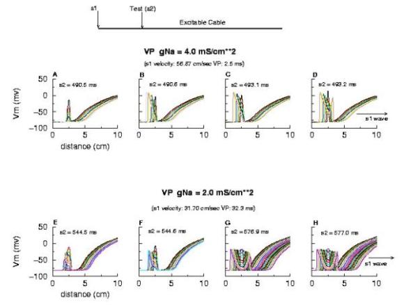
Note the right side - that the front development time for gNa = 4.0 is quite small (each trace is 5 ms apart) while when the conductance is marginal (gNa = 2.0), the front requires about 40 - 60 ms to determine if its going to succeed or collapse. Why this difference in front development time? Now, if the above hypothesis is correct, then there should be a critical excitability (or Na channel availability) associated with the transition from block to unidirectional conduction, and also with the transition from unidirectional conduction to bidirectional conduction. This is readily confirmed as shown here. Na channel availability (gNa*h*j) is plotted at the block-uni and the uni-bi boundary of the VP, and the critical channel availability is easily observed:
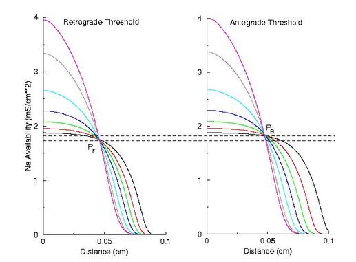
So - why the difference in thresholds? The spatial gradient of Na channel availability determines the distance (time) required for an impulse to develop into a stably propagating wave. Note that the uni-bi threshold, Pa, is greater than the block-uni threshold, Pr. This is because the block-uni threshold is determined by a front that is propagating in the retrograde direction, into MORE excitable media - whereas the uni-bi threshold is determined by a front that is propagating into LESS excitable media. These observations can be collected into a simple model of the VP where the VP measures the time required for the critical Na availability point to both pass over the stimulus field AND an extension of the electrode that reflects the distance the availability phase wave must travel in order to present the critical value, Pa at the electrode edge :
So how can these ideas help us understand the proarrhythmic potential of Na channel blockade? It has been demonstrated with the CAST study that post infarction patients have an increase in risk of sudden cardiac death if they are using drugs that have Na channel blocking properties. Antiarrhythmic drugs are "use-dependent" in that they appear to bind only to specific channel configurations. When the channel is not in one of these configurations, then the drug simply escapes from the channel. We proposed a simple model of guarded access (instead of continuous access as with most ligand-receptor interactions) (the guarded receptor hypothesis) that has been exhaustively validated in Na, Ca and K channels with a wide range of antiarrhythmic compounds. (see Molecular Pharmacology, 28:348-356, 1985; Biometrics, 44:549-559, 1988, Circulation 82:2235-2242, 1990, Circulation 84:1364-1377, 1991, PACE 20(part2): 445-454, 1997). Click for an overview of acyclic (guarded receptor) and cyclic (modulated and allosteric) models of ion channel blockade This seemingly complex behavior - reflecting both the undesired effects of premature stimulation and the proarrhythmic potential of Na channel blockade - can be readily demonstrated using the more realistic Beeler Reuter model (though we have shown this with many different cardiac models - the behavior: vulnerability and its extension linked to slowed conduction, is generic for excitable medium and even demonstratable with the chemical BZ medium). Shown here is a graph of the vulnerable period associated with differing degrees of Na channel blockade - which alters the conduction velocity. In this example the degree of antiarrhythmic drug effect was increased by increasing the rate of s1 stimulation (which increases the appearance of the bindable channel configuration). Low reexcitation intervals permitted significant unblocking between stimuli and thus minimal drug effect while high rates dramatically increase the net fraction of blocked channels. Note the linear relationship between VP and the reciprocal of the propagation velocity of the conditioning wave. Experimental verification of the alteration of the VP with Na channel blockade was demonstrated by us in Amer. J. Physiol 262:H1305-1310, 1992. In these studies, we showed that not only lidocaine, thought to be a very safe antiarrhythmic but also cocaine and synthetic opiates - which also block Na channels, extend the duration of the VP. Below is an interesting observation, that appears consistent with experiments - that use-dependent blockade prolongs the VP much more than simple reduction of G(Na), for example with TTX. It appears that while the slope of linear relationship between VP and 1/velocity holds for both use- and non use-dependent, that there is also a constant term, that is introduced with use-dependent drugs. I believe this is a result of the dynamics of blockade that occurs during the interval of front formation immediately following premature stimulation - but so far, I'm unable to pin down the mechanism. Its quite an interesting problem. Note: July 2001. Recent studies of the gradient of excitability indicate that the gradient at the s2 stimulation site is a major determinant in the VP. Since use-dependent drugs have very slow unbinding rates (otherwise, they would not be use-dependent), the gradient effect adds to the electrode effect. See the recent notes document this investigation
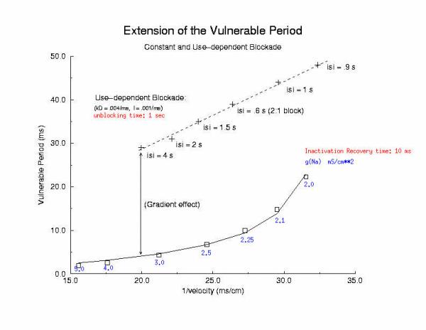
[Note August 2001 - I figure it out! The offset between the gna relationship and the use-dependent relationship is due to the additional time required to establish an antegrade propagating wave! Why? There is an asymmetry in the threshold for propagation between the retrograde and the antegrade front. The gradient links the two - and the time required to reach the antegrade threshold represents the offset between the gna changes - and use-dependent changes - and is directly proportional to the inverse gradient with is directly proportional to the unbinding time constant! ]
Two Dimensional Demonstration
The importance of the Liminal Length (Critical Nucleus)The success of spiral initiation from premature stimulation depends on will collapse. If the front is > Liminal length, then if the separation between ends is adequate to support a single circulation of the wave, then it will continue one or more rotations (see below). To meet this requirement, we simply excite a line of cells with the s2 stimulus instead of a single point. Strong point stimuli would also create a similar condition.Why the spiral tip trajectory is either circular or meandersThere is another interesting property of a spiral wave: the trajectory followed by the spiral tip. Because of the liminal length requiremnt, it is physically impossible for the spiral to rotate around a point! (Although kinetimatic approximations suggest this is possible - its a result of an infinitely steep front, with provides infinite charge for propagation - not a condition found in cardiac tissue). With a slowly propagating wave, where only a small amount of charge is available in the front, the trajectory is circular in a isotropic and uniform medium. As the charge is increased (for example, but removing a drug that blocks Na or Ca channels - or applying a drug the blocks K channels) the wave velocity increases and the diameter of the circtlar spiral tip trajectory decreases. Further increase in gNa or gCa result in decreasing the diameter of the circular core. When the circular region is approximately equivalent to the liminal region, there is a bifurcation - a transition from a circular trajectory to meandering. In electrocardiographic terms, the ecg makes a transition from monomorphic (circular - or ellipse) to polymorphic (meandering). The transition can be modulated by ion channel blockade - with Na and Ca blockade resulting in a reduction in meandering, reduced wave velocity or rotational velocity and transitions to circular or elliptical trajectories while a reduction in K channel conductance will result in increased, wave velocity, meandering and polymorphic electrocardiograms.
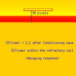
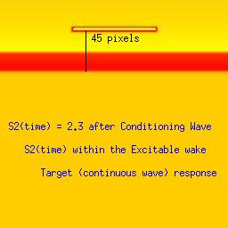
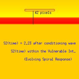
Three examples: failed front formation, successful and spiral wavesStimulation in the first example falls within the refractory interval, while the stimulus in the second example falls late, when the medium is fully recovered from the passage of the conditioning front. The third example, though, stimulation falls within the vulnerable period where the medium displays heterogeneous refractoriness and propagation is blocked in some directions.Art Winfree proposed an experiment to demonstrate the concept of vulnerability. He proposed to initiate a conditioning wave with one line of electrodes and with a set of perpendicular electrodes, to initiate the s2 or test wave. By organizing the two wave fronts perpendicular to each other, all possible vulnerable locations in a tissue or numerical preparation (in numero) would be excited with the result of a high probability of initiating reentry. Ray Ideker and his group tested this idea and called it a critical point. They also associated with it, a critical potential gradient of the s2 field, that appeared essential to initiate reentry. While these conceptual approaches to understanding the vulnerable period were quite useful within the context of the then popular "kinematic" analysis of spiral waves, they shed little new light on the fundamental nature of the vulnerable period: the interaction of the transition point between excitable and refractory tissue with the suprathreshold region of the s2 stimulus electrode. Below we demonstrate the ease with which one can induce reentry (spiral waves) if one understands the underlying mechanism. Global cross-field stimulation protocols are thus unnecessary for exploring vulnerability, and in fact, hide the underlying mechanism. Be patient with the downloads of the 3 classes of stimulus responses. Its worth it. Note the distance between the front associated with the conditioning wave and the response to the second stimulation (indicated by a black line). The geometric distance associated with a stimulus that falls within the vulnerable period (42 pixels in this example) is between that associated with a decaying response (refractory, 39 pixels) and complete excitation (45 pixels). The length of the vulnerable period in this model is only a few pixels. These are studies with a 2D Fitzhugh-Nagumo model. The first (refractory) example, stimulation is at 2.1 time units after the initial wave. The second example (fully excitable), stimulation is 2.3 time units after the initial wave. Finally, the third example (spiral) illustrates stimulation during the vulnerable period (at 2.23 time units) where the medium antegrade to the stimulation site is inexcitable, and the medium retrograde to the stimulation site is excitable. The variable load seen by the stimulation wave front at the endpoints of the resulting wave fragment drags the wave, inducing curvature and producing the spiral configuration.
From Fitzhugh-Naguma abstractions to a more realistic Cardiac Model
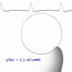

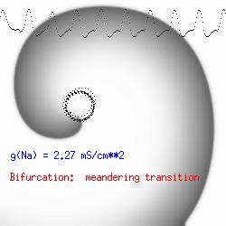
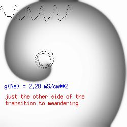
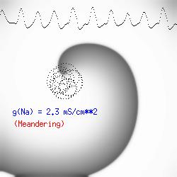
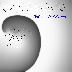
The dotted line reflects the trajectory followed by the tip of the spiral and this trajectory influences the features of the electrocardiogram. Note that increasing the conductance from 2.1 to 2.7 mS reduced the diameter of the tip trajectory as seen above and increases the variability in the individual "QRS" complexes - from monomorphic (gna = 2.1) to polymorphic (gna = 2.3). A additional small increment in the Na channel conductance which increases the available charge in the front can force a transition to a meandering spiral wave (only a 2% increase) which is the result of the wave tip trying to excite a region less than the liminal threshold (exceeds the maximum curvature defined by the liminal length criteria): To increase the degree of meandering, we increase again the Na conductance (or decrease the K channel conductance as is often accomplished with Class III antiarryhythmic drugs). The physics behind meandering and spiral formation is contained in a series of papers Josef Starobin and I published in the Biophysical Journal, 70:581-594, 1996; (Wavelet formation in excitable cardiac tissue: The role of wavefront-obstacle interactions in initiating high frequency fibrillatory-like arrhythmias); Physica D: 70:321-341, 1994 (Vulnerability in one-dimensional excitable media) and Phys Rev E: 54:430-437,1996 (Boundary-layer analysis of waves propagating in an excitable medium: Medium conditions for wave-front -- obstacle separation); In the following manuscript, we used our boundary layer analysis to predict the transition from circular tip trajectories to meandering and provided some theoretical meat to Art Winfree's elegant numerical experiments where he probed the excitable medium flower garden. Phys Rev E 55:1193-1197, 1997 (A common mechanism links spiral wave meandering and wavefront-obstacle separation), and Phys Rev E 56:3757-3760, 1997 (Boundary-layer analysis of a spiral wave core: Spiral core radius and conditions for tip separation from the boundary). The code was developed by Dr. Dmitry Romashko at the Institute of Theoretical and Experimental Biophysics in Pushchino, Moscow region - as part of our joint collaboration we refer to as our "laboratory without walls". Members include Prof. Valentin Krinsky at the Insitute of Non-linear Systems at the University of Nice, Prof. Igor Efimov at Case Western-Reserve University Prof. Vicente Perez-Munuzuri at the University of Santiago de Compostela, Prof. R. S. Reddy at the Indian Institute of Technilogy - Madras, Prof. Rubin R. Aliev, Physics Department , Vanderbilt Univ. and Prof. Dima Romashko - now in Boston, testing his skills in a new environment. Second, these videos illustrate the relationship between the electrocardiogram (ecg) and the location of the spiral tip. This illustrates one mechanism for "sustained" tachyarrhythmias that are often observed clinically. The trajectory of the spiral outlines the perimeter of a flower and is described in my research outline
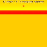
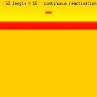
The role of the stimulus region and the liminal length:How to limit the number of spiral revolutions Here we explore with the FHN model, the responses to s2 stimulation where we vary the length of the s2 excited region - and as you will see, when the region is less than the liminal region, there is no propagated response. When the s2 excited region is > liminal length, then 1, 2 or an infinite number of reactivations are possible as shown here
Thus, by simply changing the length of the site of premature stimulation, one can vary the length of the wavelet that survives collision of the two rotating ends, thus producing 1 or 2 or continuous repetitive responses from premature stimulaion. The trick appears to be associated with the size of "pinched-off" wave after the two ends collide (following the first rotation). If the residual wavelet, following collision of the left and right spirals is < liminal region, then an additional response decays. If its greater than the liminal region, then it succeeds. By adjusting the s2 size, one basically increases the separation between the ends -thus altering the size of the pinched wavelet. Unfortunately, I've been unable to get 3 responses - either because its not possible or because my spatial discretization (dx) is too coarse. Additional studies will indicate where this will go.
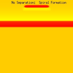
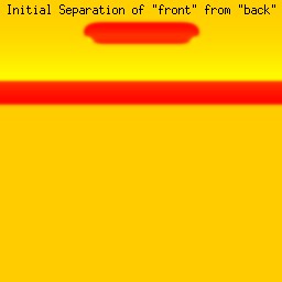
Splitting of the excitation region: the transition from spiral formation to target wave formation(click in the image for the mpg video)
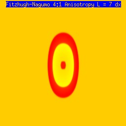
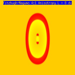
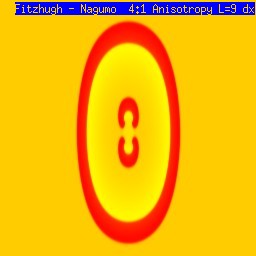
A new result: Initiating spiral waves from identical s1 and s2 sitesOne of the puzzling aspects of starting spirals in cardiac tissue is that it is usually accomplished with two consecutive stimuli arising from the same point. The question of whether one could initiate a spiral in a a spiral wave in a medium with identical cells has not been addressed (to my knowledge). Since we know that an asymetry of excitability is required for wave fragment formation, I hypothesized that we could achive the requisite asymmetry by implementing anisotropic coupling between cells. The simplest type of anisotropy is uniform anisotropy, discussed by Maddy Spach in his papers on discontinuous propagation. The main idea is that following excitation, the wave will propagate more rapidly in one direction than in an different (perhaps orthogonal) direction. Thus, the medium in the direction of slow conduction will be less excitable than the medium in the direction of fast conduction. Below are the results of 4:1 ratio of longitudinal:transverse coupling between cells. As shown below - this readily creates a vulnerable region within which stimulation can initiate spirals. Shown are 3 electrode lengths - the left, L = 7 dx and results in a decaying front (L < liminal length). The middle panel has L = 8 dx, producing a single reentrant iteration. After the first collision, the remaining fragment is < liminal region and so it collapses. The right panel, L = 9 dx and produces continuous spirals. Look at these new results and enjoy.
The liminal region, illustrated above, is the minimal excited region from which a propagating front can arise. In 2D excitation, with rectangular regions and show below, one can initiate a variety of spiral configurations - depending on which fronts (lateral or longitudinal) survive. Here, on the left, is a small excited region (L = 38 dx) from which only the longitudinal (up-down) fronts survive. On the right, is a larger excited region (L = 50 dx) from which both the longitudinal and transverse fronts survive. Step carefully through each frame and at frame 38, you'll see the separation of the fronts, and either decay or extension of the transverse fronts.
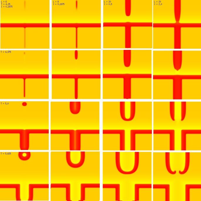
New Insights into wave splitting and the lower limit of vulnerabilityShown here is a conditioning wave that propagates from top to bottom - and a stimulus site where the width of the s2 electrode and the amplitude of the stimulus are varied. All frames (horizontally) are aligned in time and indicated in the upper left corner is the width of the electorde (x dimension) as well as the stimulus amplitude. Note that on the left, the amplitude is small as well as the electrode size are small, and only a small region far from the conditioning front is ignited. The 2nd column reveals the responses for a slightly larger (8 dx) electrode. In this case, a target wave is formed because the gradient of excitability is so small that antegrade wave formation is possible. Increasing the stimulus current to 0.5 results in a larger impulse, igniting closer to the conditioning wave, but still only a target wave forms. Note that a bridge forms that joins the fronts that propagate to the left and right respectively. It is this bridge that must be destroyed if the target is to fail and spiral evolution is to occur. Finally, with a large current, the ignited region impacts the absolute refractory region where antegrade propagation is impossible - front splitting occurs (i.e. the bridge cannot form and so two spirals evolve from the 2 wave fragments.
 This work is licensed under a Creative Commons License. C. Frank Starmer |
 Note
also that has increasing the inhibitory current (less negative values)
further reduces the rest potential (the constant regions either side of the
critical nucleus.
Note
also that has increasing the inhibitory current (less negative values)
further reduces the rest potential (the constant regions either side of the
critical nucleus.
 Here, a disturbance in a uniformly excitable media propagates away from
the site of excitation. The excited area exceeds that of the
critical nucleus and expands away from the initial disturbance..
The blue trace - representing the amplitude of the
inhibitory current. The red trace is the membrane potential.
Here, a disturbance in a uniformly excitable media propagates away from
the site of excitation. The excited area exceeds that of the
critical nucleus and expands away from the initial disturbance..
The blue trace - representing the amplitude of the
inhibitory current. The red trace is the membrane potential.
 When the inhibitory current (blue)
is non uniform, in this case a simple gradient, then excitability
varies linearly along the cable (grad = 0.005). When
the medium is disturbed such that the critical nucleus requirement is exceeded
in the more excitable direction but not met in the less excitable direction,
unidirectional propagation results. The gradient can be considered as the
first term in a Taylor series, so that this approach can be viewed as
an approximation of an arbitrary distribution of excitability.
When the inhibitory current (blue)
is non uniform, in this case a simple gradient, then excitability
varies linearly along the cable (grad = 0.005). When
the medium is disturbed such that the critical nucleus requirement is exceeded
in the more excitable direction but not met in the less excitable direction,
unidirectional propagation results. The gradient can be considered as the
first term in a Taylor series, so that this approach can be viewed as
an approximation of an arbitrary distribution of excitability.