|
|


Next: Generating Random Variables
Up: Chi-Square Goodness of Fit
Previous: Chi-Square Goodness of Fit
Index
Click for printer friendely version of this HowTo
Consider a binomial random variable
 with
mean with
mean
 and variance and variance
 . From the Central
Limit Theorem, we know that . From the Central
Limit Theorem, we know that
 has an
approximately a standard Normal(0,1) distribution for large values of has an
approximately a standard Normal(0,1) distribution for large values of
 . Since the square of a
standard normal random variable has a chi-square distribution with one
degree of freedom, . Since the square of a
standard normal random variable has a chi-square distribution with one
degree of freedom,  is approximately is approximately  . .
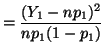
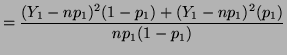
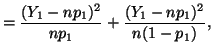
Now consider the random variable  which has a binomial which has a binomial distribution and let
 and and
 . Then . Then
and since
we have
where has a chi-square distribution with 1 degree of freedom.
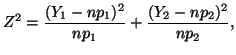
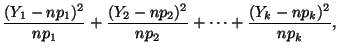
In general, for  random variables random variables  , where , where
 ,
with corresponding expected values ,
with corresponding expected values  , a statistic measuring the
``closeness'' of the observations to their expectations is the sum: , a statistic measuring the
``closeness'' of the observations to their expectations is the sum:
which has a chi-square distribution with  degrees of freedom.
This is because we know that the sum of all of the probabilities, degrees of freedom.
This is because we know that the sum of all of the probabilities,
 , must equal 1, and thus we can derive , must equal 1, and thus we can derive  by
subtracting the first probabilities from 1. by
subtracting the first probabilities from 1.
Allele Frequenciesno_title
The population is said be in Hardy-Weinberg equilibrium for a given
gene if it is:
- Stable with respect respect to the allele and genotype frequencies
of interest. That is, allele frequencies do not change from
generation to generation.
- The genotype frequencies in the progeny produced by random
mating among parents is determined solely by the allele frequencies of
the parents.
In other words, if, for a particular gene A with alleles A and A
and A , and the allele frequencies in the parents are , and the allele frequencies in the parents are  A A and A and A (and thus (and thus  or or  ), than the percentage of
offspring with the genotype AA ), than the percentage of
offspring with the genotype AA , AA , AA and AA and AA . .
Table:
Observed genotypes at the MN blood group gene locus for
individuals in a human population. Source:
Plagiarized from Michael D. Purugganan, class notes.
| Genotype |
Observed |
| AA |
22 |
| AA |
216 |
| AA |
492 |
|
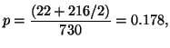
Given the data in Table 3.7.2, we can calculate the
observed allele frequencies. That is,
and
With values for  and and  , we can now calculate how many individuals
with each class of genotype we would expect if the population was in
Hardy-Weinberg Equilibrium. The results of this calculation are in
Table 3.7.3. , we can now calculate how many individuals
with each class of genotype we would expect if the population was in
Hardy-Weinberg Equilibrium. The results of this calculation are in
Table 3.7.3.
Table 3.7.3:
Both observed and expected genotypes at the MN blood group
gene locus for
individuals in a human population.
| Genotype |
Observed |
Expected |
| AA |
22 |
23.14 |
| AA |
216 |
213.60 |
| AA |
492 |
493.26 |
|
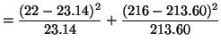
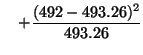
Now that we have both observed and expected values for each class of
genotype, we can calculate a chi-square test statistic. That is,
Now all we need to do is compare this value to that from a chi-square
distribution. The trick, however, is determining how many degrees of
freedom there are. Here we have three different categories, or
genotypes, and each one has an associated probability of membership.
However, two of these probabilities are dependent on one of them.
That is, since the probability of having the genotype
AA
 and the probability of having the
genotype AA and the probability of having the
genotype AA
 . Thus, since there is only one
linearly independent probability, the degree of freedom is 1. . Thus, since there is only one
linearly independent probability, the degree of freedom is 1.
We can now use Octave to determine the probability our hypothesis is
correct:
octave:2> 1 - chisquare_cdf(0.086, 1)
ans = 0.76933
So, since we usually fail to reject the hypothesis that the data comes from
our model if the probability is more than 5 percent (and in this case
it is 77 percent, see Figure 3.7.2), we will not
reject the hypothesis that that alleles for the MN blood type gene are
in Hardy-Weinberg Equilibrium.
Figure:
The area under the graph that represents the p-value, the probability
our hypothesis that the Locus for the MN blood group is in
Hardy-Weinberg Equilibrium is correct. Since the p-value/area is so large (77
percent) we will accept our hypothesis (or Fail to Reject our hypothesis).
![\includegraphics[width=3in]{chi_square2}](img580.png) |

Next: Generating Random Variables
Up: Chi-Square Goodness of Fit
Previous: Chi-Square Goodness of Fit
Index
Click for printer friendely version of this HowTo
Frank Starmer
2004-05-19
| |