|
|


Next: Conclusion
Up: Linear Models
Previous: Hypothesis Testing
Index
Click for printer friendely version of this HowTo
Linear Models with
Multiple Dependent Variables
Suppose the observations, or dependent variables,  s, are vectors
with s, are vectors
with  correlated characteristics instead of single variables, as
would be the case of multiple observations made on the same
individual. A random sample of correlated characteristics instead of single variables, as
would be the case of multiple observations made on the same
individual. A random sample of  of these vectors could be arranged
in a rectangular array to form an of these vectors could be arranged
in a rectangular array to form an
 matrix Y, where
the first row of Y is the vector of characteristics observed on
the first individual, the second row is the vector observed on the
second individual and so on. matrix Y, where
the first row of Y is the vector of characteristics observed on
the first individual, the second row is the vector observed on the
second individual and so on.
Assuming that the -dimensional
observation vector has a multivariate normal distribution, and that
the observations vectors are independent, we can extend the
univariate model developed in Sections 3.13.1
through3.13.5 to encompass the correlated variables.
The model now appears as:
 |
(3.13.22) |
which looks exactly like the univariate general linear model in
Equation 3.13.3, except in this case, Y is an
matrix and
 is an is an
 matrix. The matrix
X, the design matrix, is the same matrix of known constants that
appeared in the univariate model. The
hypothesis can be generalized to: matrix. The matrix
X, the design matrix, is the same matrix of known constants that
appeared in the univariate model. The
hypothesis can be generalized to:
 |
(3.13.23) |
where C is an
 matrix U is a matrix U is a
 matrix, and
 is an is an
 matrix and C
and U are arbitrary matrices designed to yield the appropriate
hypothesis. matrix and C
and U are arbitrary matrices designed to yield the appropriate
hypothesis.
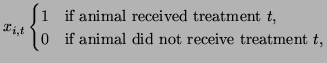
Multiple Regressionno_title
A series of animals were studied where cardiac output and mean blood
pressure were measured while heart rate and respiration were varied.
The data from this study can be found in
Appendix C.1. We will model with data with the
formula:
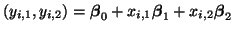 |
(3.13.24) |
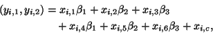
where
 mean blood pressure of the mean blood pressure of the  -th animal, -th animal,
 cardiac output of the -th animal, cardiac output of the -th animal,
 respiration rate of the i-th animal, respiration rate of the i-th animal,
 heart rate of the i-th animal. heart rate of the i-th animal.
Thus,
and
Some questions that we might ask about this data are
- Does respiration rate affect cardiac output and mean blood pressure?
- Does heart rate affect cardiac output and mean blood pressure?
To answer the first question, we test the hypothesis that the respiration
rate regression coefficients are zero:
We can convert this hypothesis into matrix form using
Equation 3.13.25 by defining C and U such
that
which yields:
To answer the second question, we test the hypothesis that the heart
rate coefficients are zero:
for which
Since, in general, these two tests will not be independent, we should
make them simultaneously. To do this, let
Using Equation 3.13.25, this yields:
We are now ready to use the multivariable version of the general
linear models program found in Appendix
 Hotelling T Hotelling T no_title no_title
Hotelling T tests allow us to run simultaneous paired  -tests on
pairs of characteristics. Consider, in this case, that we have
measured mean blood flow, mean blood pressure, cerebro-vascular
resistance in a series of experimental subjects both before and after
the administration of epinephrine. Using a Hotelling T we can
answer the question: Did the drug change the blood flow, pressure and
resistance significantly? -tests on
pairs of characteristics. Consider, in this case, that we have
measured mean blood flow, mean blood pressure, cerebro-vascular
resistance in a series of experimental subjects both before and after
the administration of epinephrine. Using a Hotelling T we can
answer the question: Did the drug change the blood flow, pressure and
resistance significantly?
The model for this experiment is thus
where
- blood flow before
- blood pressure before
 resistance before resistance before
- blood flow after
- blood pressure after
- resistance after
where the subscript 'b' refers to a measurement taken before the
treatment and the subscript 'a' refers to a measurement taken after.
To answer our question about whether the drug changed blood flow,
pressure and resistance, we ask if the parameters for before and
after measurements have changed. Thus, we form the hypothesis:
This leads us to define C and U as:
so that
or, in other words,
The output from our program is...
Multivariate ANOVAno_title
A series of twenty-four animals were studied by dividing them into six
groups according to their diet and sex. The cardiac output, heart
rate, and initial body weight of the animals were measured. Since body
weight was thought to affect the level of response, it is considered a
covariate. Cardiac output and heart rate are both dependent
variables. Our model is thus,
where
and
To test if cardiac output and heart rate vary with sex, we construct
the contrast matrices:
and
Thus, our hypothesis is3.27:
Next: Conclusion
Up: Linear Models
Previous: Hypothesis Testing
Index
Click for printer friendely version of this HowTo
Frank Starmer
2004-05-19
| |
![\begin{displaymath}
{\bf C} =
\left[
\begin{array}{ccc}
0 & 1 & 0
\end{array}\r...
... =
\left[
\begin{array}{cc}
1 & 0\\
0 & 1
\end{array}\right],
\end{displaymath}](img1047.png)
![\begin{displaymath}
{\bf C} =
\left[
\begin{array}{ccc}
0 & 0 & 1
\end{array}\r...
... =
\left[
\begin{array}{cc}
1 & 0\\
0 & 1
\end{array}\right].
\end{displaymath}](img1053.png)
![\begin{displaymath}
{\bf C} =
\left[
\begin{array}{ccc}
0 & 1 & 0\\
0 & 0 & 1
...
... =
\left[
\begin{array}{cc}
1 & 0\\
0 & 1
\end{array}\right].
\end{displaymath}](img1054.png)
![\begin{displaymath}
{\bf C} \boldsymbol{\beta} {\bf U} =
\left[
\begin{array}{c...
...
=
\left[
\begin{array}{cc}
0 & 0\\
0 & 0
\end{array}\right].
\end{displaymath}](img1055.png)
![\begin{displaymath}
\boldsymbol{\beta} =
\left[
\begin{array}{cccccc}
\beta_{\...
...begin{array}{c}
1\\
1\\
1\\
\vdots\\
1
\end{array}\right],
\end{displaymath}](img1059.png)
![\begin{displaymath}
{\bf C} = [1]
\textrm{ and }
{\bf U} =
\left[
\begin{array}...
...\\
-1 & 0 & 0\\
0 & -1 & 0\\
0 & 0 & -1
\end{array}\right],
\end{displaymath}](img1063.png)
![\begin{displaymath}
{\bf U} =
\left[
\begin{array}{cc}
1 & 0\\
0 & 1
\end{array}\right].
\end{displaymath}](img1072.png)
![\begin{displaymath}
\left[
\begin{array}{c}
(\beta_{1,1} + \beta_{2,1} + \beta_{...
...eta_{4,2} + \beta_{5,2} + \beta_{6,2})
\end{array}\right]
= 0.
\end{displaymath}](img1073.png)
![$\displaystyle = \left[ \begin{array}{cc} y_{1,1} & y_{1,2} \vdots & \vdots y_{n,1} & y_{n,2} \end{array} \right],$](img1041.png)
![$\displaystyle = \left[ \begin{array}{ccc} 1 & x_{1,1} & x_{1,2} \vdots &\vdots & \vdots 1 & x_{n,1} & x_{n,2} \end{array} \right],$](img1043.png)
![$\displaystyle = \left[ \begin{array}{cc} \beta_{0,1} & \beta_{0,2} \beta_{1,1} & \beta_{1,2} \beta_{n,1} & \beta_{n,2} \end{array} \right].$](img1045.png)
![$\displaystyle \left[ \begin{array}{ccc} 0 & 1 & 0 \end{array} \right] \left[ \b...
... \end{array} \right] \left[ \begin{array}{cc} 1 & 0 0 & 1 \end{array} \right]$](img1048.png)
![$\displaystyle \left[ \begin{array}{cc} \beta_{1,1} & \beta_{1,2} \end{array} \right] \left[ \begin{array}{cc} 1 & 0 0 & 1 \end{array} \right]$](img1050.png)