Next: Generating Normally Distributed Random
Up: Generating Random Variables
Previous: Generating Random Variables
Index
Click for printer friendely version of this HowTo
Suppose you want to do some
experiments that explore the stochastic nature of a process. For
example, you
incorporate a random variable into a model. The first thing you
must do is
create some observations that have variation according to the
distribution of the random variable. Most often, the method used to do
this is to invert the Cumulative Distribution Function (described
below) and feeding it a random number between 0 and 1.3.3
It is possible to convert from
a uniform(0,1) random variable to something nonuniform, and also the
reverse. Although this may sound backward, and in fact is, we will
start by describing how to do the reverse.
Figure 3.8.1 shows a typical exponential
distribution, which starts
at 1 and ends near zero. The Cumulative Distribution Function (or
CDF) for the same distribution can be used to map an exponential
random variable to a uniform(0,1) variable and is shown in Figure 3.8.2. The
CDF for any distribution is defined as the cumulative probability from
the smalled number in the domain to a specific point in the distribution,  .
That is,
.
That is,
 . If
. If  is distributed by the exponential function
 , then
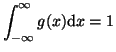
Since the total area under any distribution is always 1, that is for
any distribution,  ,
it is clear that the CDF for any distribution can be used to map any
random variable from that distribution to a number between 0 and 1.
Since no part in the CDF will be visited any more than any other part,
the mapping is to a uniform(0,1) distribution.
,
it is clear that the CDF for any distribution can be used to map any
random variable from that distribution to a number between 0 and 1.
Since no part in the CDF will be visited any more than any other part,
the mapping is to a uniform(0,1) distribution.
Figure:
PDF of an exponential process with rate = 1:

![\includegraphics[width=3in]{pdf}](img589.png) |
Figure:
CDF of an exponential process with rate = 1:
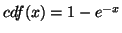
![\includegraphics[width=3in]{cdf}](img590.png) |
To map a uniform(0,1) random variable to an
exponential distribution you simply do the reverse. That is, use the
inverse of the exponential distribution CDF,
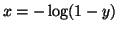 , and apply it to a
uniform(0,1) variable.
, and apply it to a
uniform(0,1) variable.
Here is some Octave code that demonstrates this transformation
(see Figure 3.8.3 for the histogram):
octave:1> uniforms = rand(50, 1);
octave:2> exps = -log( 1 - uniforms);
octave:3> hist(exps) # plot histogram
Figure:
A histogram of 50 exp(1) random variables
![\includegraphics[width=3in]{hist1}](img592.png) |
This method, in general works very well for the subset of distributions that
are formed by transforming uniform random variables. These include the
Beta, Gamma, Chi-squared, F, Exponential, Double Exponential and
Weibull distributions. Other distributions rely on tricks to
generate random variables. Despite the fact that this text attempts
to avoid describing tricks at all costs, due to their utility we will
list two of them.
Next: Generating Normally Distributed Random
Up: Generating Random Variables
Previous: Generating Random Variables
Index
Click for printer friendely version of this HowTo
Frank Starmer
2004-05-19