|
|


Next: Anatomy of a model
Up: How to create a
Previous: Algebraic Models
Index
Click for printer friendely version of this HowTo
Ordinary Differential Equations
Models can be built from words or from equations. We usually start with
a word model, or qualitative model,
just to get the central concepts organized. But qualitative models
are difficult to explore and sooner or later, we find ourselves translating
actions in our word models into equations that describe the
quantitative results of these actions. Tools such as matlab and octave make
quantitative models easy to explore. Simple command line tools, series and tf also give us a means for exploring algebraic
models.
series generates a sequence of numbers of length num_terms
from begin to end
This sequence of numbers can then be piped into tf, a tool for
evaluating an algebraic expression and these
results can be piped into a plot tool. Thus, a you can set up an easy
pipeline with a shell command like this:
shell> series begin end num_terms |
       tf "algebraic_expression" | plot
and the moral of the story is that numerical tools enable the model to be used as a simulation of the real
phenomena and certain hypotheses can be tested against it. Word
models, on the other hand, can describe a process, but are not so
easily converted into computer programs and tested.
Differential equations come in all flavors and sizes. They basically have
the form
where  can be linear, nonlinear, have constant coefficients or
variable coefficients. Often times can be linear, nonlinear, have constant coefficients or
variable coefficients. Often times  is a function of is a function of  . That
is, . That
is,  . The highest order derivative in the equation
determines the order of the differential equation. Differential
equations with only a single
independent variable are called Ordinary Differential Equations
(ODEs). Those with more than one independent variable are called
Partial Differential Equations (PDEs), due to the fact that the
derivatives are partial derivatives. The solution to a differential
equation is the unknown function . The highest order derivative in the equation
determines the order of the differential equation. Differential
equations with only a single
independent variable are called Ordinary Differential Equations
(ODEs). Those with more than one independent variable are called
Partial Differential Equations (PDEs), due to the fact that the
derivatives are partial derivatives. The solution to a differential
equation is the unknown function  that you have the derivative
for. While this may seems backward, in nature, we can observe how
something changes over time, and thus, we can fit a derivative to this
data. From this derivative, we then try to determine the original function. that you have the derivative
for. While this may seems backward, in nature, we can observe how
something changes over time, and thus, we can fit a derivative to this
data. From this derivative, we then try to determine the original function.
A differential equation describes changes in one variable relative to
another variable, and as such, solutions to differential equations are
functions that describe the ups and downs of a function. For example,
 or or
 where is the dependent variable and
is the independent variable. The differential equation: where is the dependent variable and
is the independent variable. The differential equation:
 |
(2.4.1) |
is an equation that says the change in for a certain change in is
negatively proportional to the value of . In other words, when
is large, the slope of the solution
(d/d) is negative and proportional
to (the proportionality constant is  ). As becomes smaller,
the slope becomes smaller. ). As becomes smaller,
the slope becomes smaller.
The solution to Equation 2.4.1 is
 |
(2.4.2) |
where the constant  is determined
by the ``initial condition'', the value of when is determined
by the ``initial condition'', the value of when  . If . If
 , then , then
 ; if ; if
 , then , then
 .
The solution of the differential equation, produces a ``class'' of similar
solutions, and a particular member of that class is identified by the
initial condition. .
The solution of the differential equation, produces a ``class'' of similar
solutions, and a particular member of that class is identified by the
initial condition.
Building an ODEno_title
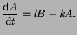
Consider a simple chemical reaction. We have a substance, , that
spontaneously converts to  with a rate, with a rate,  , while
spontaneously converts to with a rate, , while
spontaneously converts to with a rate,  .
Schematically, we can notate this with the equation: .
Schematically, we can notate this with the equation:
From this, we can describe the change in as the proportion of
that converts into minus the proportion of that changes into
. That is,
 |
(2.4.3) |
If we enforce conservation of mass so that the combined mass of
and is always constant,
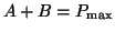 , we can
now rewrite the Equation 2.4.3 as , we can
now rewrite the Equation 2.4.3 as
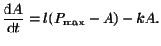 |
(2.4.4) |
Without explicitly finding a solution to Equation 2.4.4, we
can determine what it will be when it is at equilibrium. That is to
say, we can determine what proportion of
 needs to
be comprised of
such that the amount of converting to is the same as the
amount of converting to , or needs to
be comprised of
such that the amount of converting to is the same as the
amount of converting to , or
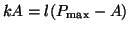 .
We do this by setting the slope of to zero and solving for : .
We do this by setting the slope of to zero and solving for :
Thus, if
then the amounts of and will not change.
Now that we know what the equilibrium is, it is interesting to look at
the general solution to Equation 2.4.4
because the
equilibrium plays a large role in it. Equation 2.4.4
can be solved using various methods. In Example
2.10.3.1 we show how to use an integrating factor to
solve for  and the result is: and the result is:
Notice what happens as gets larger and larger. If we take
the limit, we get
and thus, the system converges on the equilibrium. The exponential
term simply causes the difference between the initial condition, the
amount of at time , or  , the equilibrium to become
smaller and smaller as time passes. , the equilibrium to become
smaller and smaller as time passes.

Two Componants as Oneno_title
Now, consider a two component reaction,
This is
called a second order reaction because the reaction rate depends on the
concentration of two components, and . However, under certain
conditions, it can be treated as a first order reaction, like in Example 2.4.0.1. When the concentration
of or is essentially infinite, and there is a small concentration
of the other component, then we have a pseudo first order reaction.
Here we will show how this is possible from the differential equation.
We start with a 2nd order equation where the rate of formation is
determined by the concentration of [] and [],
We assume that s
collide with s at a rate determined by the temperature of the reaction
and that a certain fraction of the collisions will result in making
a  . If the availability of is infinite so that its concentration
never changes, the rate constant can be rewritten as a
pseudo rate constant . If the availability of is infinite so that its concentration
never changes, the rate constant can be rewritten as a
pseudo rate constant  : :
and this allows us to treat the second order reaction as if it were
first order. This assumption, that is infinite, is often
reasonable when is some sort of drug compound and is a cellular
receptor for this compound.
Next: Anatomy of a model
Up: How to create a
Previous: Algebraic Models
Index
Click for printer friendely version of this HowTo
Frank Starmer
2004-05-19
| |


![$\displaystyle A(t) = \frac{P_{\textrm{max}}}{(1+\frac{k}{l})} - \left[\frac{P_{\textrm{max}}}{(1+\frac{k}{l})} - A(0)\right]e^{-(l+k)t}.$](img129.png)