Next: Markov and Stochastic Models
Up: Methods for Solving ODEs
Previous: Using Matrix Algebra
Index
Click for printer friendely version of this HowTo
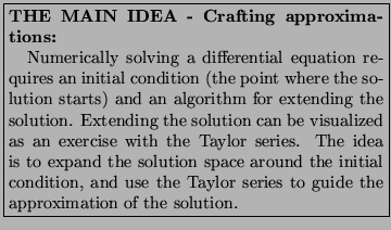
Finding an analytical soltion to a differential equation is not always a
practical option. Numerical approximations lead to solutions that are
much more readily available, however, there are a number of
issues related to the approximation that should be understood.
The trick to constructing a viable
numerical solution of a differential is identifying a reliable
approximation of the derivative and then selecting a step size that
results in both a stable and physically meaningful solution.
Errors acquired during the construction of a numerical
solution arise from two sources: roundoff and truncation.
Roundoff error arises from the limited precision of
computer arithmetic. The problem is compounded in that
the binary representation of many fractions is
irrational, enhancing the effects of the roundoff error. For example,
1/10 is irrational in the binary system whereas
1/8 is rational. For this reason, we often choose discretization intervals
that are powers of 1/2 instead of powers of 1/10.
The second source of error is called truncation error. This error
arises when we make discrete approximations of continuous functions.
This error can be, to a certain extent, limited by making the
step-sizes in the discrete function as small as possible. The Taylor
series, which provided a means for creating approximate functions,
also allows us to evaluate the truncation error.
We often evaluate the quality of a numerical solution
by estimating the error incurred with our functional approximations.
Forward Euler Methodno_title
We start with a simple first order initial value problem (IVP)
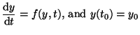 |
(2.10.17) |
where f(y,t) is some linear or non-linear function of y and t and
 is the initial value of y at time
  .
.
Finding approximate values for points other than is simply a
matter of figuring out what step size,  , of the independent
variable,
, of the independent
variable,  to use.
Figure 2.10.8 shows the idea of extending the solution using
a forward Euler solution.
to use.
Figure 2.10.8 shows the idea of extending the solution using
a forward Euler solution.
Figure:
The general idea for extending a solution using
a forward Euler method.
![\includegraphics[width=3in]{numerical_step}](img428.png) |
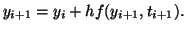
The strategy is to start at a point and extend the solution with a step
size, h. So we start at  , compute the amount of y we must
add,
, compute the amount of y we must
add,
 and then use this point to repeat the algorithm:
-

-
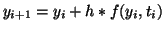
This is called the Forward Euler method because the right hand side,
 is evaluated at the initial point. Now, is this a good method? We'll
now look at a Taylor expansion of our method, and estimate the error and
the stability of the solution. By stability we mean will the numeric solution
reflect the analytic solution for arbitrary conditions (like step size and
nature of the function, ).
is evaluated at the initial point. Now, is this a good method? We'll
now look at a Taylor expansion of our method, and estimate the error and
the stability of the solution. By stability we mean will the numeric solution
reflect the analytic solution for arbitrary conditions (like step size and
nature of the function, ).
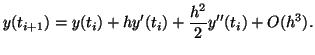
Now, using the Taylor series, Equation 2.2.1, we will expand
 around
  and assess the truncation error:
 |
(2.10.18) |
The three left terms represent the truncated Taylor series (Euler's Method)
while the right two terms represent the local truncation error. We
are assuming that  and thus, the
 term indicates that all terms that follow in the series will
be less than
term indicates that all terms that follow in the series will
be less than  . We see
that the method is accurate to order , and not the higher order
terms (
. We see
that the method is accurate to order , and not the higher order
terms ( or ), so we say that its first order
accurate.
or ), so we say that its first order
accurate.
In order to detrmine how stable this method is for approximating an
ordinary differential equation, we simply try to detrmine whether or
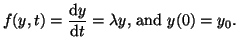
not it will converge or diverge for large values of  . For example,
we will use a simple function:
. For example,
we will use a simple function:
 so that
Using this to replace the function, , in Equation
2.10.19, we have
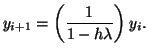
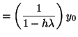
Now, if you start at the initial value,  , and repeatedly apply the
above equation, you'll find that
, and repeatedly apply the
above equation, you'll find that
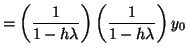
We call the multiplier,
 the amplification factor. Clearly
if
the amplification factor. Clearly
if
 then the solution will blow up after a few steps.
Thus, the solution is only stable when
then the solution will blow up after a few steps.
Thus, the solution is only stable when
 , since the step
size, , can never be negative itself.
, since the step
size, , can never be negative itself.

Backward Euler Methodno_title
The Forward Euler method approximates the points  by starting from
some initial point, and moving to the right using the
derivatave as calculated at
by starting from
some initial point, and moving to the right using the
derivatave as calculated at  . An alternative to this is to
start from and move to the right using the derivative as
calculated at .
That is, we evaluate the function, at
. An alternative to this is to
start from and move to the right using the derivative as
calculated at .
That is, we evaluate the function, at
 . To
do to this, we rewrite the second formula in the numerical approximation as
. To
do to this, we rewrite the second formula in the numerical approximation as
 |
(2.10.19) |
Now we let
and solve for and find that
and thus,
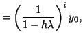
Starting at the initial condition,  we see that
and the amplification factor is now  for all values of
(again, since the step size, , can never be negative). Thus,
this method only provides a stable solution when
.
This method is referred to as an implicit method, since the function is
evaluated at a solution point, yet to be determined. For all linear
functions,
for all values of
(again, since the step size, , can never be negative). Thus,
this method only provides a stable solution when
.
This method is referred to as an implicit method, since the function is
evaluated at a solution point, yet to be determined. For all linear
functions,  , a nice iterative equation can be determined. When is
non-linear, then typically the function is linearized (with a Taylor
series, of course) and each step in the solution is interated until
the fuction is well approximated by the Taylor approximation.
, a nice iterative equation can be determined. When is
non-linear, then typically the function is linearized (with a Taylor
series, of course) and each step in the solution is interated until
the fuction is well approximated by the Taylor approximation.
Leap Frog Methodno_title
The error associated with the simple Euler method can be improved by
realizing that for both the forward (explicit) and backward (implicit)
Euler methods, there is an asymmetry between approximating the derivative
and evaluating the function. For the explicit method, the function
(right hand side) is evaluated at the left side of the derivative while
for the implicit method, is evaluated at the right side of the
derivative. The price for this approximation is that we now need to
know two values of y  and
and  before we can extend the solution to the next point.
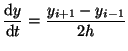
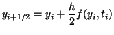
We can also evaluate at the midpoint of the
derivative, and this is called the Leap Frog Method.
before we can extend the solution to the next point.
We can also evaluate at the midpoint of the
derivative, and this is called the Leap Frog Method.
so that
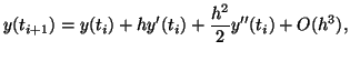
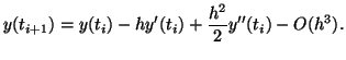
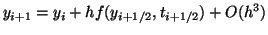
As before, we can evaluate the accuracy of this strategey by comparing
to the Taylor expansion of the function. We first make a Taylor
approximation for both and :
and
Now, subtracting the two series, we see that the the 2nd order terms
cancel. Thus, this method is 2nd order accurate.
Runge-Kutta Methodno_title
The solution accuracy can be further improved by building a strategy
around the leap-frog method and the forward Euler method. This
mixture results in a Runge-Kutta method that has even more accuracy.
The half step is computed with the forward Euler method and then
the full step is computed with the leap-frog method.
 |
(2.10.20) |
 |
(2.10.21) |
Like the leap frog method, this method is 2nd order accurate. The Runge-Kutta
method applies to a class of methods where intermediate steps are taken.
For example, we can make 4 evaluations and make a procedure that is 4th order
accurate:
 |
(2.10.22) |
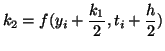 |
(2.10.23) |
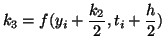 |
(2.10.24) |
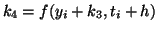 |
(2.10.25) |
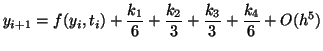 |
(2.10.26) |
This procedure is a very popular procedure, and will usually do you right. It
is safe, accurate, and except for really wierd models, will provide reliable
solutions.
Fortunately, octave (matlab) has some very nice tools for solving odes
for us. Here are two little scripts just to indicate what is needed.
The first segment defines the ode as a function,
in this case du/dt = u(1-u)(u-a) + stim
where stim is the stimulation that forces the system to switch from one
stable state to another:
> more trigger.m

function xdot=trigger(x,t)

% Trigger threshold for stim = 0.25 is 1.039 time units

xdot = zeros(1,1);
a = 0.25;
stim = 0;

if t < 1.039
   stim = 0.25;
end

xdot(1) = x(1)*(1.0-x(1))*(x(1)-a) + stim;

endfunction
To to actually solve the ode, we execute the following piece of code
within matlab which calls the ode solver: lsode and then plots the results
> more fhn_trigger.m

t = linspace(0,50,400);

%x0 = [0.0; 0.0];
x0 = [0.0];

y = lsode("trigger",x0,t);

plot(t,y);

z = [t' y];
save -ascii plot.dat z;
Next: Markov and Stochastic Models
Up: Methods for Solving ODEs
Previous: Using Matrix Algebra
Index
Click for printer friendely version of this HowTo
Frank Starmer
2004-05-19