|
|


Next: Solving Constrained Optimization Problems
Up: Likelihood Ratio Tests
Previous: Likelihood Ratio Tests
Index
Click for printer friendely version of this HowTo
Likelihood ratio tests are ratios of distributions using parameters
derived using both constrained and unconstrained maximum likelihood.
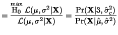
That is, the likelihood ratio test,  is, is,
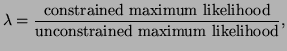 |
(3.10.1) |
where the constraint placed on the MLEs in the numerator is the
hypothesis that you want to test. In Section 3.9 we saw
how to solve for un-constrained MLEs. In the following examples we
will see how to solve for and work with constrained MLEs.
The closer the ratio in Equation 3.10.1 is to 1, the
more probable that the hypothesis that we are testing is true. The
closer this ratio is to 0, the less likely that the hypothesis is correct.
Almost all statistical tests can be derived from likelihood ratio
tests. As usual, the best way to get a grasp of this concept is to
see a few examples.
no_titleno_title
Imagine that we have a set of data, X, as described in
Example 3.9.2.1, and we want to test to see if
 . That is, let the null hypothesis be H . That is, let the null hypothesis be H
 .
In Example 3.9.2.1 we derived the
unconstrained maximum likelihood estimates for .
In Example 3.9.2.1 we derived the
unconstrained maximum likelihood estimates for  and and  (see Equations 3.9.2 and 3.9.3).
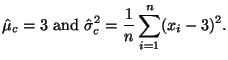
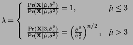
In this case, to derive the constrained MLEs we simply substitute in the
value 3 wherever
(see Equations 3.9.2 and 3.9.3).
In this case, to derive the constrained MLEs we simply substitute in the
value 3 wherever  is used, including the derivation of is used, including the derivation of
 . Thus,
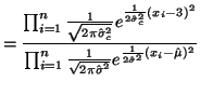
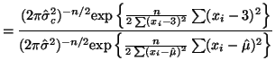
and our likelihood ratio test is: . Thus,
and our likelihood ratio test is:

no_titleno_title
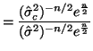
Imagine that we have the same set up as we had in
Example 3.10.1.1, only this time, the hypothesis that we want
to test is  . In this case, when . In this case, when
 , we let , we let
 . However, when . However, when
 , then , then
 . Thus, . Thus,
Notice that the LRT for
 is the same as the
LRT for is the same as the
LRT for
 when
. when
.
Next: Solving Constrained Optimization Problems
Up: Likelihood Ratio Tests
Previous: Likelihood Ratio Tests
Index
Click for printer friendely version of this HowTo
Frank Starmer
2004-05-19
| |