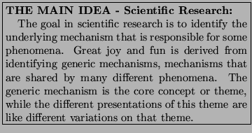
Click for printer friendely version of this HowTo Introduction What is an example of a core concept and some variations? Frank's research over the past 20 years has focused on reentrant cardiac arrhythmias and the potential role antiarrhythmic drugs might play in amplifying the potential for triggering reentrant arrhythmias. Under normal condition, the membrane potential of a group of pacemaker cells oscillates with a frequency of about 1/min. Each time the membrane potential exceeds a threshold, neighboring cells are excited and a wave of excitation propagates away from the pacemaker region. Because the heart is a closed surface, this wave will eventially collide with itself and thereby is extinguished (due to a property called refractoriness). A reentrant arrhythmia is one where the excitation wave circulates around the heart without colliding with another wave and therefore is capable of reexciting the heart. Clearly, a continuous front can never become reentrant. However a discontinuous front can evolve into a reentrant process [16]. The variations of the theme of discontinuous fronts are all the different ways one can make a discontinuous wave: by premature excitation, by collision of a front with an obstacle, by excessive front curvature and by encountering non-uniform refractory states. Each variation has specific detail that is required for the mechanism to successfully function within a specific environment. 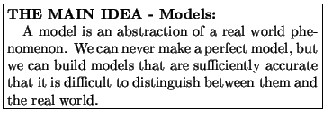Typically, one begins by creating a model of a specfic event or phenomenon. However, over time, one might notice that the model applies to other events or phenomena and can be used to answer questions that are completely unrelated to the original intent, thus, demonstrating the potential for generalizing the model. To be able to demonstrate that a model, as representing some physical mechanism, generalizes to describe processes in many different settings is the greatest thrill possible. The main challenge in biology is identifying processes, mechanisms and developing an understanding of the minimally complex representation. But before starting to model, we ask, about what features the model must represent. For example, we view a living organism as requiring 6 essential processes: metabolism (converting nutrients to energy sources), translation (translating an electrical signal to motion), signaling (transfering the representation of an event from one place to another), replication (duplicating something) and regulation, If we model an organism, then probably these features must be included in the model. Such models are quite useful, because we can use the model of one entity as a template for investigating and characterizing another. For example, at the level of the nucleus. expression could be considered as replication, signaling could reflect the initiators and terminators of expression, metabolism could reflect the supply of raw materials to the expression system etc. 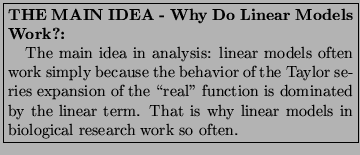For all these complexities, though, it seems that linear models are adequate to describe many processes. Not that these processes are inherently linear. Rather most likely, the range over which we can explore them is small, and the processes appears linear. 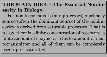Figure: A Saturating Process: A frequently occurring nonlinearity in biological systems A dose-response curve of a saturable receptor reaction where $U =$ unoccupied sites and $O =$ occupied sites. In the case of a finite number of receptors, with a huge drug concentration, all receptors are occupied - and increasing the concentration does nothing. Similarly, at very small concentrations, no receptors are occupied - and at intermediate concentrations, some receptors are occupied, leading to the sigmoid shaped dose-response curve: represented by $b = 1/(1 + l/kD)$ where b is the fraction of bound receptors, l is the reverse rate constant, k is the forward rate constant and D is the drug concentration. When D is small, b = 0 and when D is large, b = 1. Below we'll derive this relationship exactly. Thus (see below) estimating parameters derived from linear models is an important statistical tool. We'll derive a simple least squares procedure and hypothesis testing concept that is readily generalized to nonlinear and categorical data models. In addition, the fact that many nonlinearities are derived from saturable processes results in simple linear approximations of the saturable process: 3 lines - one for low concentrations, one for intermediate concentrations, and one for near saturable concentrations. Unless you happen to be operating near the knees of a saturable process, linear models work really well. One of the main products of statistical theory is that parametric procedures (which assume normally distributed variations) usually give the same answers as their non-parametric sisters. This is due to the central limit theorem. The central limit theorem says that sums of random variates are asymptotically normally distributed. My numerical studies indicate that when you have 7 or 8 terms in the series, then asymptotic normality rules the day. Thus, we never worry about the underlying distribution (well almost never) because we are analyzing sums of random variates (mean, variance etc) which are asymptotically normal (or chi square for sums of squared normal variants). Model building can be based on algebraic equations or differential equations. When do we use which? The main idea with differential equations can be best viewed by comparing with algebraic equations. Solving algebraic equations results in finding points that satisfy the equations, while solving differential equations results in finding functions that satisfy the equations. Here we show how differential equations arise in ordinary problems and how to solve a simple first order linear ODE (ordinary differential equation). With these tools, you can run over any boulder. Modeling is simply translating a physical process into some equations that describe the physical process. Thus, the idea is to get a mental image of the process to be modeled, then using basic physical and chemical concepts, write the ODEs or PDEs that describe the process. Click for printer friendely version of this HowTo

>