Next: Methods for Solving ODEs
Up: How to create a
Previous: A Single Cell
Index
Click for printer friendely version of this HowTo
Now lets use the Taylor series and an arbitrary ordinary differential
equation and explore some potentially interesting behavior. First
there are two classes (at least) of model builders. Class one
is interested in building a full model of some process that is as
realistic as possible. Class two is interested in building a minimal
model, one that captures essential behavior and upon which, one can
add more and more realism and ask: How does this altered the behavior
of the minimal model?
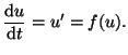
We start with the simplest ordinary differential equation:
 |
(2.9.1) |
and ask the question - what is the behavior of this equation as
we increase the complexity of f(u)? The Taylor series is a way
to methodically add complexity (by adding successive terms)
in order to more realisticly
represent a characterization of some unknown function, f(u).
Starting with the constant term, we can analyze the properties
of the ODE and get some ideas about how adequately it represents
some process of interest.
So we start with
The values of  and its derivatives are simply constants
so that the Taylor series is simply a power series in
and its derivatives are simply constants
so that the Taylor series is simply a power series in  .
So lets rewrite the series as
.
So lets rewrite the series as
and start our analysis. For convenience, we will set  to zero.
The properties of  are not interesting. The solutions
are lines of varying slope, where the slope is determined by the value
of
are not interesting. The solutions
are lines of varying slope, where the slope is determined by the value
of  .
.
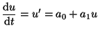
Including the first two terms makes the solution
space a bit more interesting:
 |
(2.9.2) |
This has a single equilibrium where  and the equilibrium is
located at
and the equilibrium is
located at
 . Moreover, the equilibrium is
unstable2.5 if
. Moreover, the equilibrium is
unstable2.5 if  as shown in Figure 2.9.1. When there is a
disturbance that moves the phase point,
as shown in Figure 2.9.1. When there is a
disturbance that moves the phase point,  to the left,
then we see that
to the left,
then we see that  which pushes the phase point away from the equilibrium. Similarly
when the disturbance moves the phase point to the right,
which pushes the phase point away from the equilibrium. Similarly
when the disturbance moves the phase point to the right,  which pushes the phase point to the right, again away from the equilibrium.
Figure:
Linear nullcline for Equation 2.9.2. Here the slope = 1/2 and
the root is unstable.
![\includegraphics[width=3in]{linear}](img312.png) |
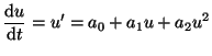
Now, we add the quadratic term and have
 |
(2.9.3) |
We assume that all the constants are such that there are 2
intersections with the line in the  plane. If there
were no intersections, then again, the behavior is not interesting.
So these two intersections represent 2 equilibria, one stable and
one unstable. See Figure 2.9.2.
plane. If there
were no intersections, then again, the behavior is not interesting.
So these two intersections represent 2 equilibria, one stable and
one unstable. See Figure 2.9.2.
Figure:
Quadratic nullcline for Equation 2.9.3. The left root is unstable,
the right root is stable
![\includegraphics[width=3in]{quadratic}](img315.png) |
Next we add the cubic term and have
 |
(2.9.4) |
Now, in the plane, we have constants,  such that there
are 3 intersections with . and depending on the values of
the , we either have two stable and one unstable equilibrium or
we have two unstable and one stable equilibrium. Figure 2.9.3
displays the cubic where we have two stable and one unstable
equilibrium.
such that there
are 3 intersections with . and depending on the values of
the , we either have two stable and one unstable equilibrium or
we have two unstable and one stable equilibrium. Figure 2.9.3
displays the cubic where we have two stable and one unstable
equilibrium.
Figure:
Cubic nullcline for Equation 2.9.4. The left root is unstable,
the right root is stable
![\includegraphics[width=3in]{cubic_null}](img318.png) |
Now what is interesting about this from a biological modeling
perspective? Many biological processes behave like switches. A
neuron is either in the rest state or the excited state. A
cardiac cell is either in the rest state or the excited state - and
translated to muscle, the muscle is either resting or contracted.
We can even look at transcription. Either the gene is being
expressed or not.
All of these process have in common, switch-like behavior. From
a modelling perspective, it means that the minimal complex model
for describing a switch requires a cubic function on the right
hand side of the ODE which means that only nonlinear systems
can represent switching behavior. Also, the middle, unstable
equilibrium, represent a threshold. So all switches must have a
threshold, and we should be able to design experiments to reveal
the threshold. Now, a distraction. If there is diffusive coupling
between switches and all are initially in the same state, then
as one switch is forced to change states, the switches to the
left and right can potentially be induced to switch (if the
diffusive element forces the local value of u to exceed the
switching threshold) and the result will be a propagating wave.
It is exciting to see the verification of a theoretical argument
(above taylor expansion of an arbitrary function) in real biological
systems. In figure 2.9.4 we see the current voltage relationship
measured in an isolated rabbit cardiac atrial cell. Using the voltage
clamp procedure, the potential was gradually increased from negative to
positive and the current associated with each potential was recorded.
The resultant i/v is a quasi-steady state and does not accurately reflect
the dynamics of a cardiac (or nerve) cell. Nevertheless, the cubic
nature is clearly seen (due to calcium channels).
Figure:
Current voltage relationship obtained from voltage clamp studies of
cultured rabbit cardiac atrial cells. Note the cubic-like behavior
![\includegraphics[width=3in]{iv}](img319.png) |
Now the fun part of modeling is
to link the cubic function to some real mechanism. In the
case of cardiac and neuronal cells, the cubic function represent
the instantaneous current-voltage relationship of the cell. We are
unsure what the cubic function represents in a gene expression
system.
Next: Methods for Solving ODEs
Up: How to create a
Previous: A Single Cell
Index
Click for printer friendely version of this HowTo
Frank Starmer
2004-05-19